这篇文章是继我昨天完成的文章 “Elasticsearch：ES|QL 函数及操作符” 的另外一篇文章。我将继续使用之前文章 “Elasticsearch：ES|QL 快速入门” 中的例子来结合 ES|QL 函数来做更进一步的展示。希望能对之前的文章做一个更进一步的展示。在这里，我将主要使用 Dev Tools 来进行展示。

特别值得注意的是：在进行如下的例子之前，你需要至少安装 Elastic Stack 8.11 及以上版本。

准备数据

我们还是仿照之前的文章里的例子来进行展示。我个人比较喜欢较少的文档做为例子来进行展示。这里的原因是，文档较少，容易设置，同时容易看清。只要能说明问题，就是好的例子。针对之前的 DSL 查询，我们可以参阅以前的文章 “开始使用 Elasticsearch （2）”。里面展示的文档也不是很多。

我们先到 Dev Tools 里打入如下的命令：

PUT sample_data
{
  "mappings": {
    "properties": {
      "client.ip": {
        "type": "ip"
      },
      "message": {
        "type": "keyword"
      }
    }
  }
}

PUT sample_data/_bulk
{"index": {}}
{"@timestamp": "2023-10-23T12:15:03.360Z", "client.ip": "172.21.2.162", "message": "Connected to 10.1.0.3", "event.duration": 3450233}
{"index": {}}
{"@timestamp": "2023-10-23T12:27:28.948Z", "client.ip": "172.21.2.113", "message": "Connected to 10.1.0.2", "event.duration": 2764889}
{"index": {}}
{"@timestamp": "2023-10-23T13:33:34.937Z", "client.ip": "172.21.0.5", "message": "Disconnected", "event.duration": 1232382}
{"index": {}}
{"@timestamp": "2023-10-23T13:51:54.732Z", "client.ip": "172.21.3.15", "message": "Connection error", "event.duration": 725448}
{"index": {}}
{"@timestamp": "2023-10-23T13:52:55.015Z", "client.ip": "172.21.3.15", "message": "Connection error", "event.duration": 8268153}
{"index": {}}
{"@timestamp": "2023-10-23T13:53:55.832Z", "client.ip": "172.21.3.15", "message": "Connection error", "event.duration": 5033755}
{"index": {}}
{"@timestamp": "2023-10-23T13:55:01.543Z", "client.ip": "172.21.3.15", "message": "Connected to 10.1.0.1", "event.duration": 1756467}

我们可以把上面的最后的 bulk 命令运行两遍，这样会有更多的数据来进行展示。

我们有两种方法可以运行查询：

在 Dev Tools 中运行
在 Discover 中运行

我们为刚才创建的索引 sample_data 创建 data view：

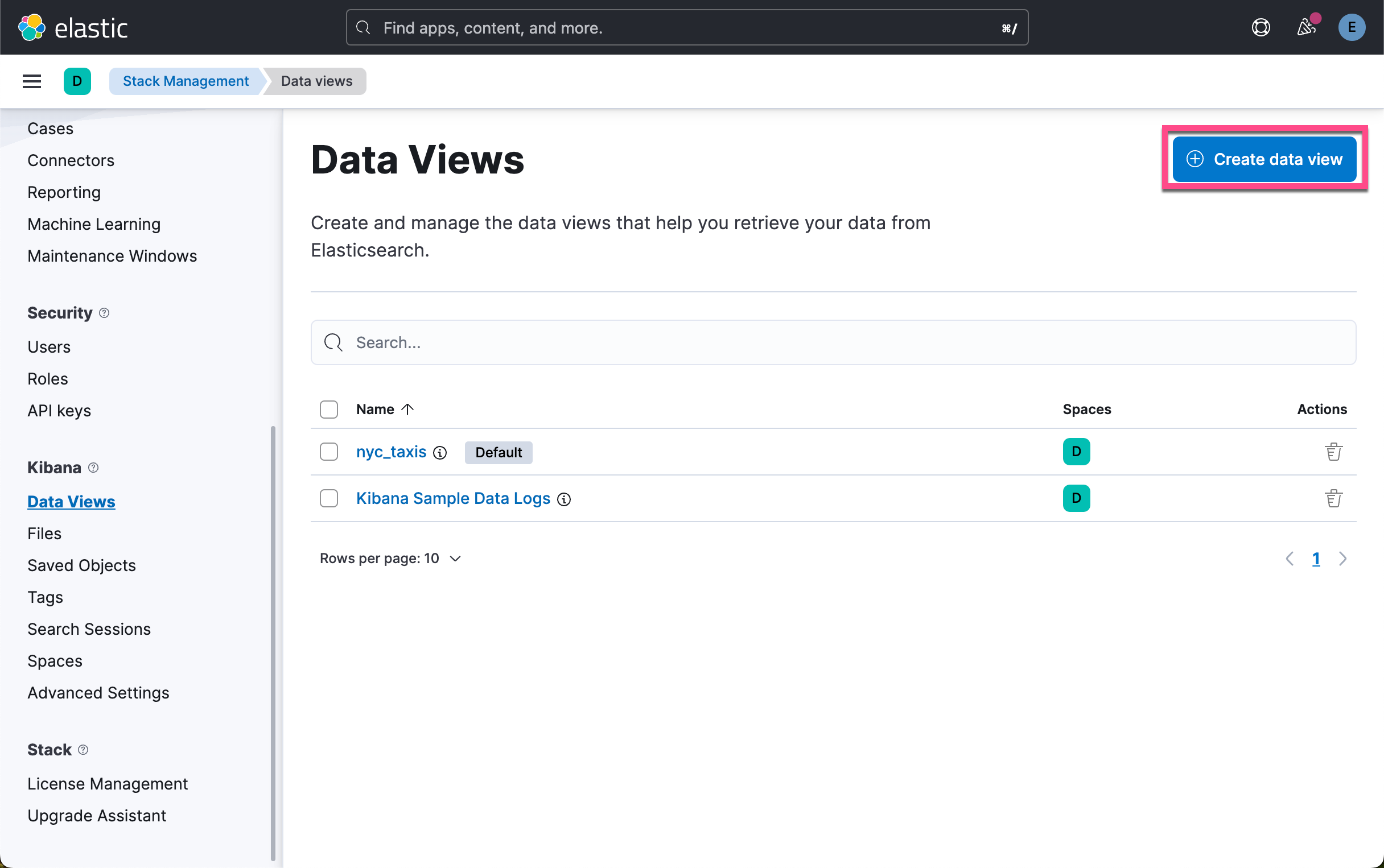
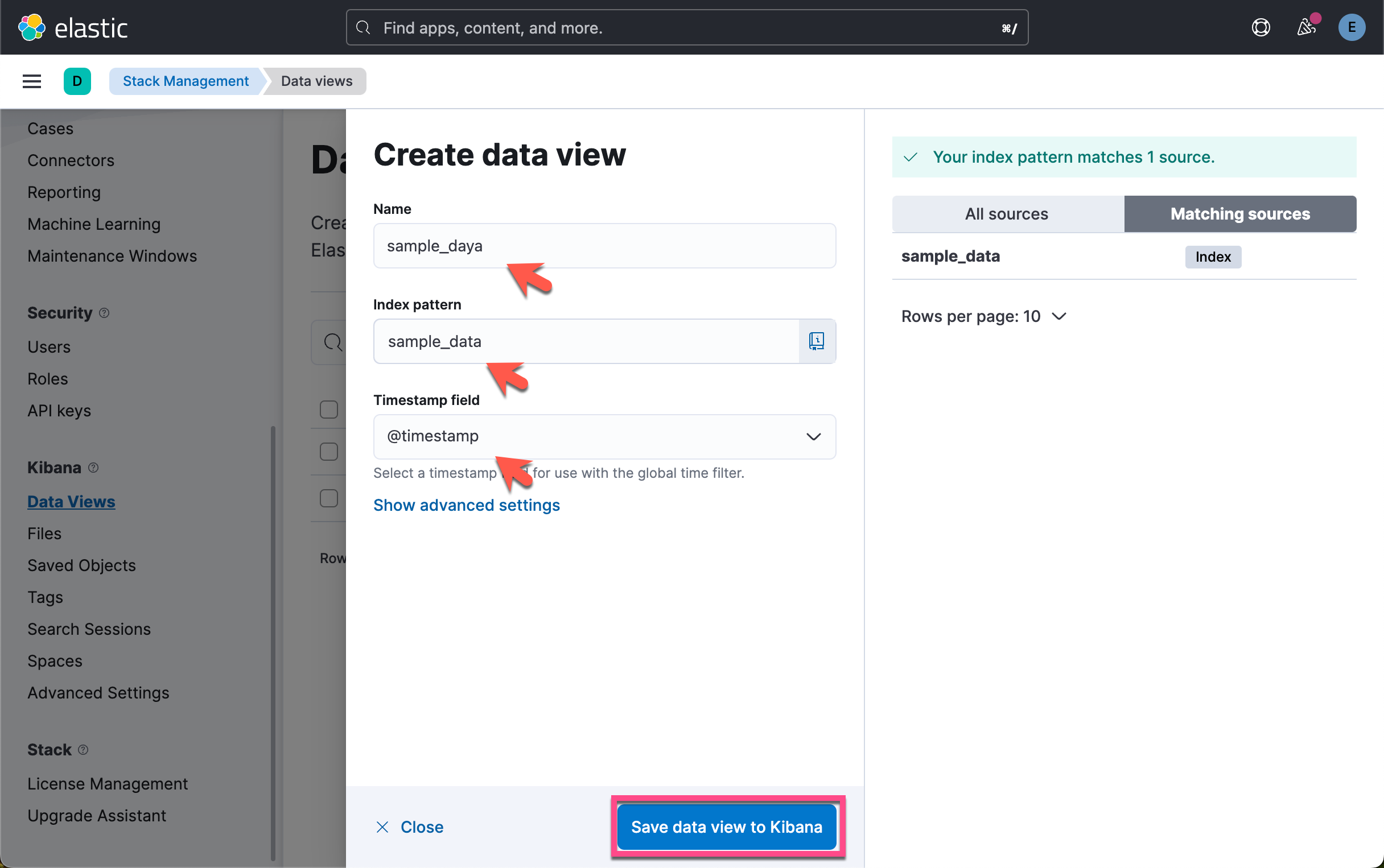
虽然这个操作针对 Dev Tools 里的查询是不必要的。

在 Dev Tools 里进行查询

基本语法

ES|QL 查询由一个源命令组成，后跟一系列可选的处理命令，并用竖线字符分隔：|。例如：

source-command
| processing-command1
| processing-command2

查询的结果是最终处理命令生成的表。

为了便于阅读，本文档将每个处理命令放在一个新行中。但是，你可以将 ES|QL 查询编写为一行。以下查询与前一个查询相同：

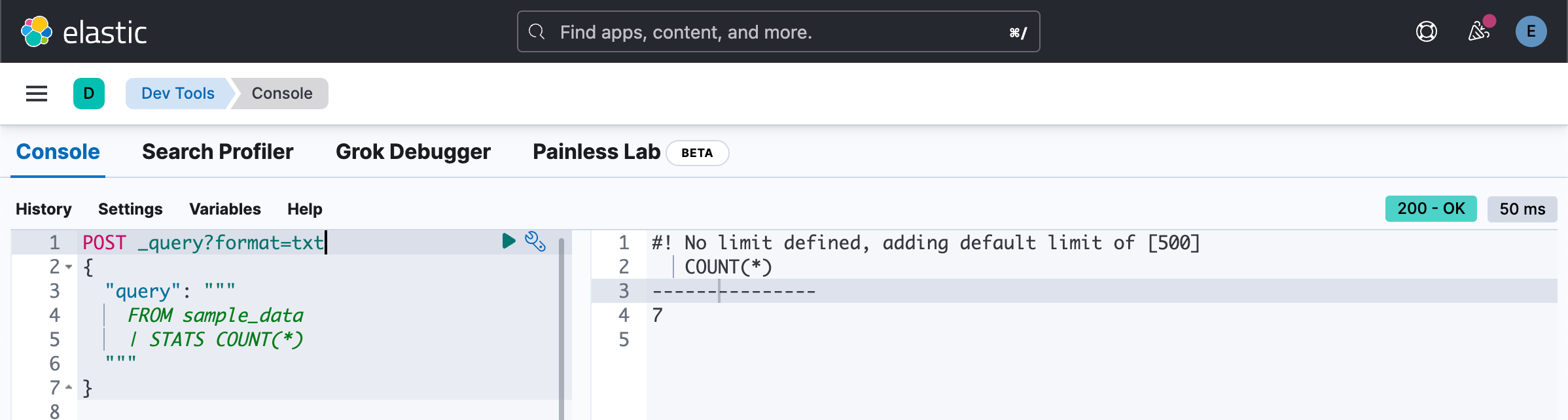
source-command | processing-command1 | processing-command2

如下命令得到总的文档个数：

POST _query?format=txt
{
  "query": """
    FROM sample_data
    | STATS COUNT(*)
  """
}

它类似于之前的如下命令：

GET sample_data/_count

ES|QL 源命令

ES|QL 源命令会生成一个表，通常包含来自 Elasticsearch 的数据。

ES|QL 支持以下源命令：

FROM
ROW
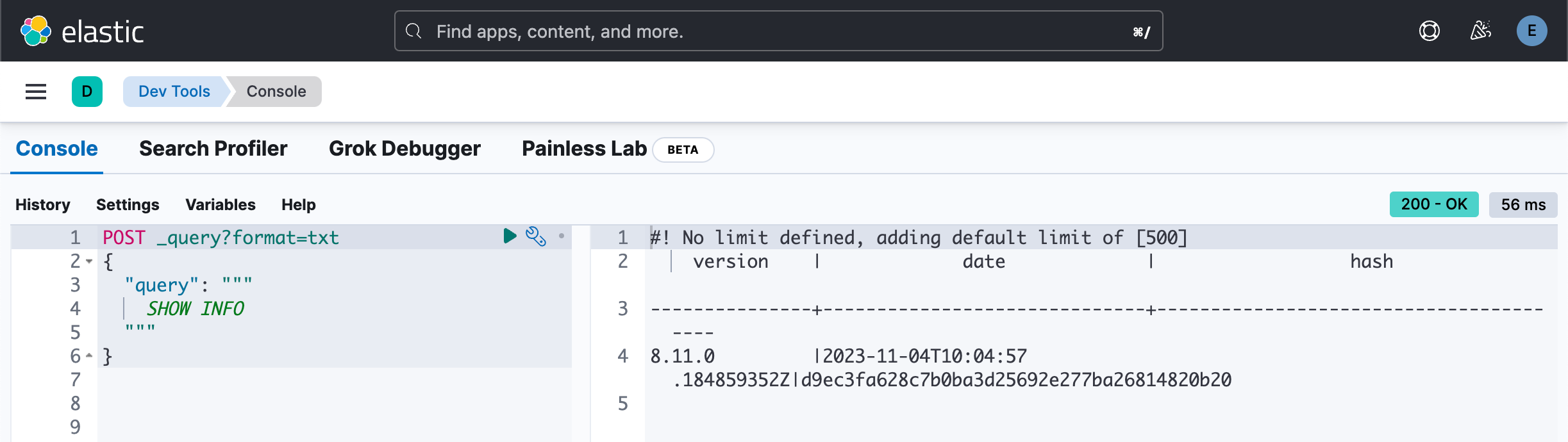
SHOW <item>

POST _query?format=txt
{
  "query": """
    SHOW INFO
  """
}

上面的命令和下面的命令是一样的结果。它不分大小写：

POST _query?format=txt
{
  "query": """
    show info
  """
}

我们可以有如下的注释：

POST _query?format=txt
{
  "query": """
    SHOW INFO // Get the info
    /* Then get rid of the warning and only select the version field */
    | LIMIT 1
    | KEEP version
  """
}

我们在哪里放置 pipe 符号呢？

POST _query?format=txt
{
  "query": """
    SHOW INFO | LIMIT 1 | KEEP version
  """
}

POST _query?format=txt
{
  "query": """
    SHOW INFO | 
    LIMIT 1 | 
    KEEP version
  """
}

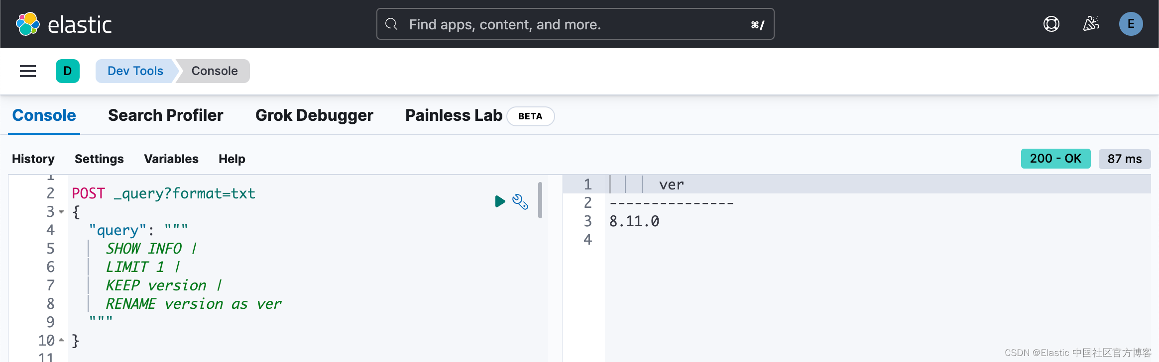
我们也可以使用 RENAME 命令来修改字段的名称：

POST _query?format=txt
{
  "query": """
    SHOW INFO | 
    LIMIT 1 | 
    KEEP version |
    RENAME version as ver
  """
}

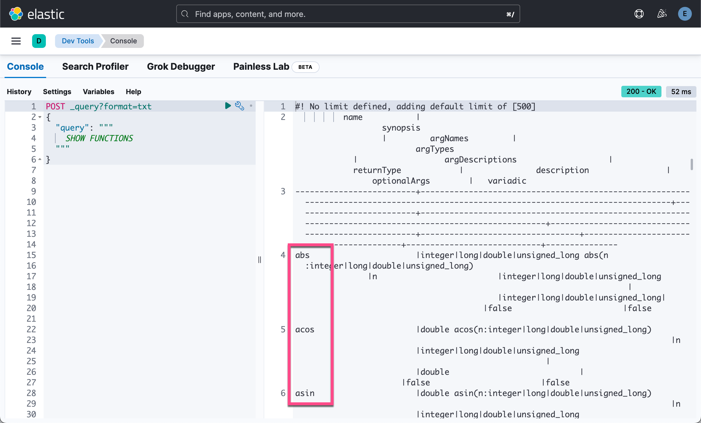
POST _query?format=txt
{
  "query": """
    SHOW FUNCTIONS
  """
}

我们需要在 Kibana 的界面中，进入到 Dev Tools。通常一个 ES|QL query API 的命令格式是这样的：

POST /_query?format=txt
{
  "query": """
  """
}

在两组 """ """之间输入实际的 ES|QL 查询。例如：

POST /_query?format=txt
{
  "query": """
    FROM sample_data
  """
}

你可以链接处理命令，并用竖线字符分隔：|。每个处理命令都作用于前一个命令的输出表。查询的结果是最终处理命令生成的表

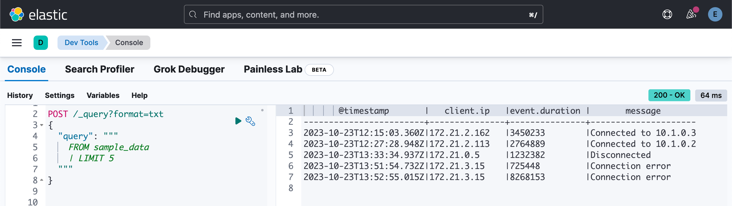
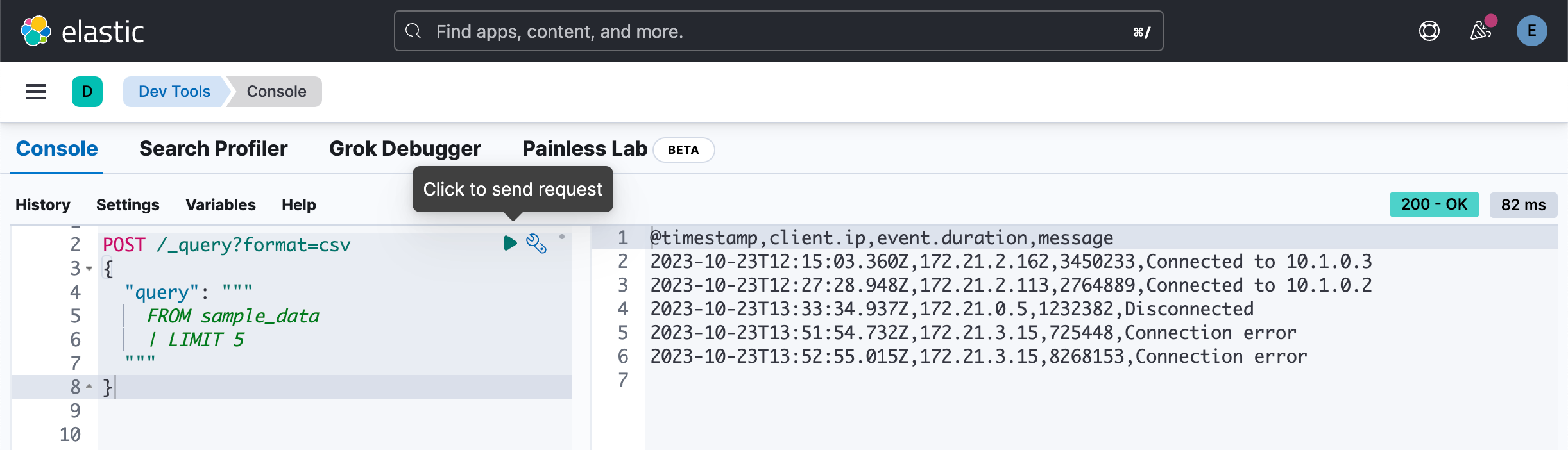
我们可以通过使用 LIMIT 来限定返回的文档数：

POST /_query?format=txt
{
  "query": """
    FROM sample_data
    | LIMIT 5
  """
}

这个相当于 DSL 的如下查询：

GET sample_data/_search?size=5

如果未指定，LIMIT 默认为 500。无论 LIMIT 值如何，单个查询都不会返回超过 10,000 行。

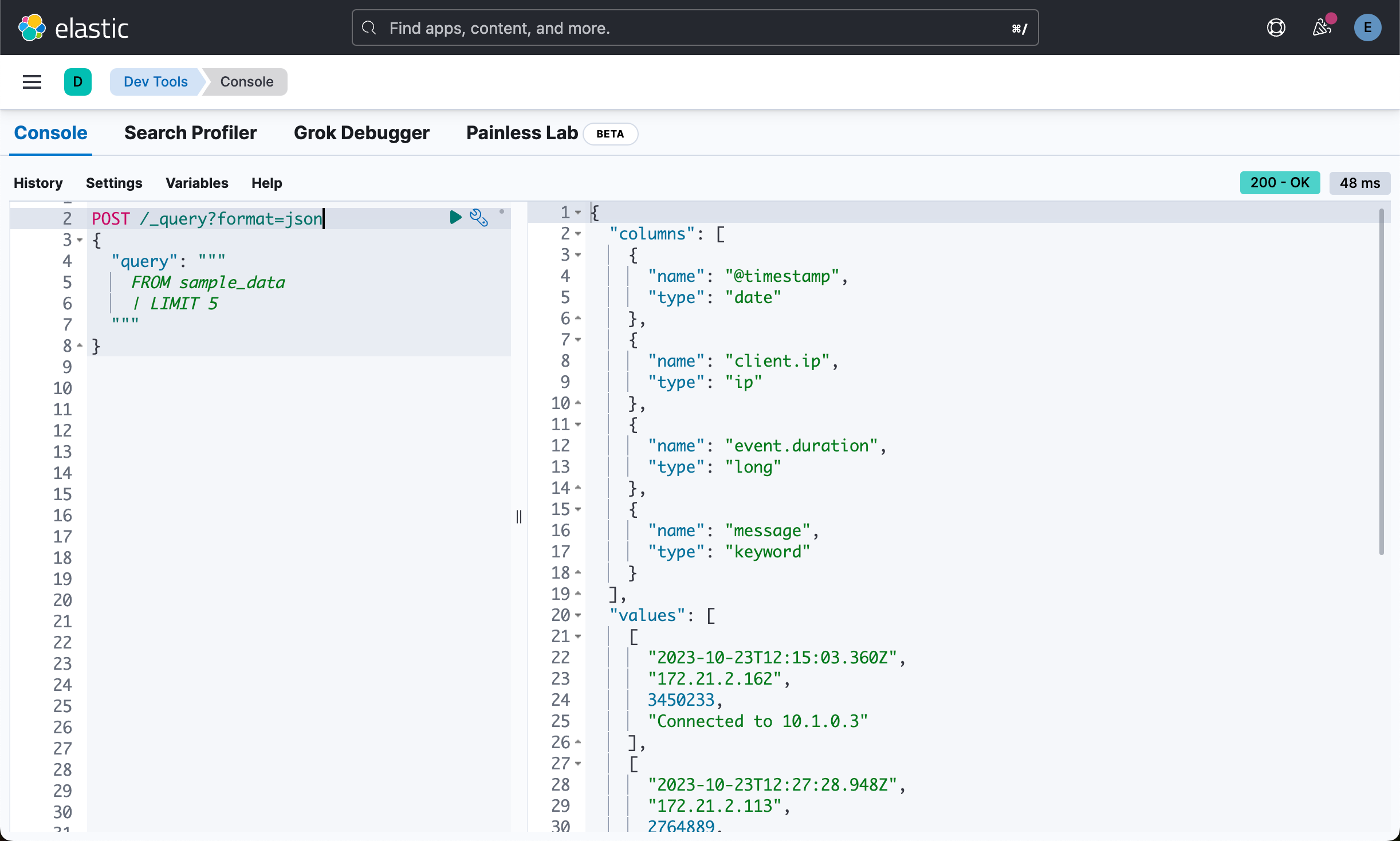
在上面我们使用 format=txt 的格式来进行返回。我们可以使用 JSON 的格式：

POST /_query?format=json
{
  "query": """
    FROM sample_data
    | LIMIT 5
  """
}

同样我们也可以使用 CSV 格式作为输出：

POST /_query?format=csv
{
  "query": """
    FROM sample_data
    | LIMIT 5
  """
}

上述命令类似于 DSL：

GET sample_data/_search
{
  "size": 5
}

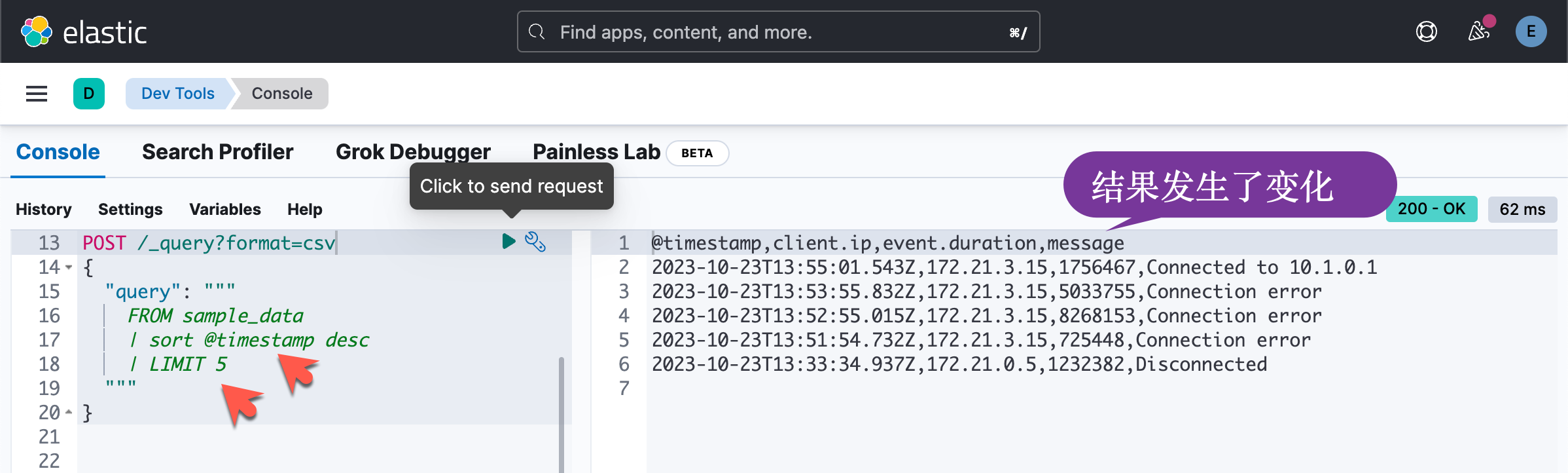
在输出的时候，我们可以使用字段来进行排序，比如按照时间字段 @timestamp 来进行降序排序：

POST /_query?format=csv
{
  "query": """
    FROM sample_data
    | LIMIT 5
    | sort @timestamp desc
  """
}

这个相当于 DSL 的如下查询：

GET sample_data/_search?size=5
{
  "sort": [
    {
      "@timestamp": {
        "order": "desc"
      }
    }
  ]
}

但是结果不完全一样。更加贴近的结果是：

POST /_query?format=csv
{
  "query": """
    FROM sample_data
    | sort @timestamp desc
    | LIMIT 5    
  """
}

我们运行如下的查询：

POST _query?format=txt
{
  "query": """
    FROM sample_data
    | WHERE client.ip = "172.21.2.162"
    | LIMIT 10
  """
}

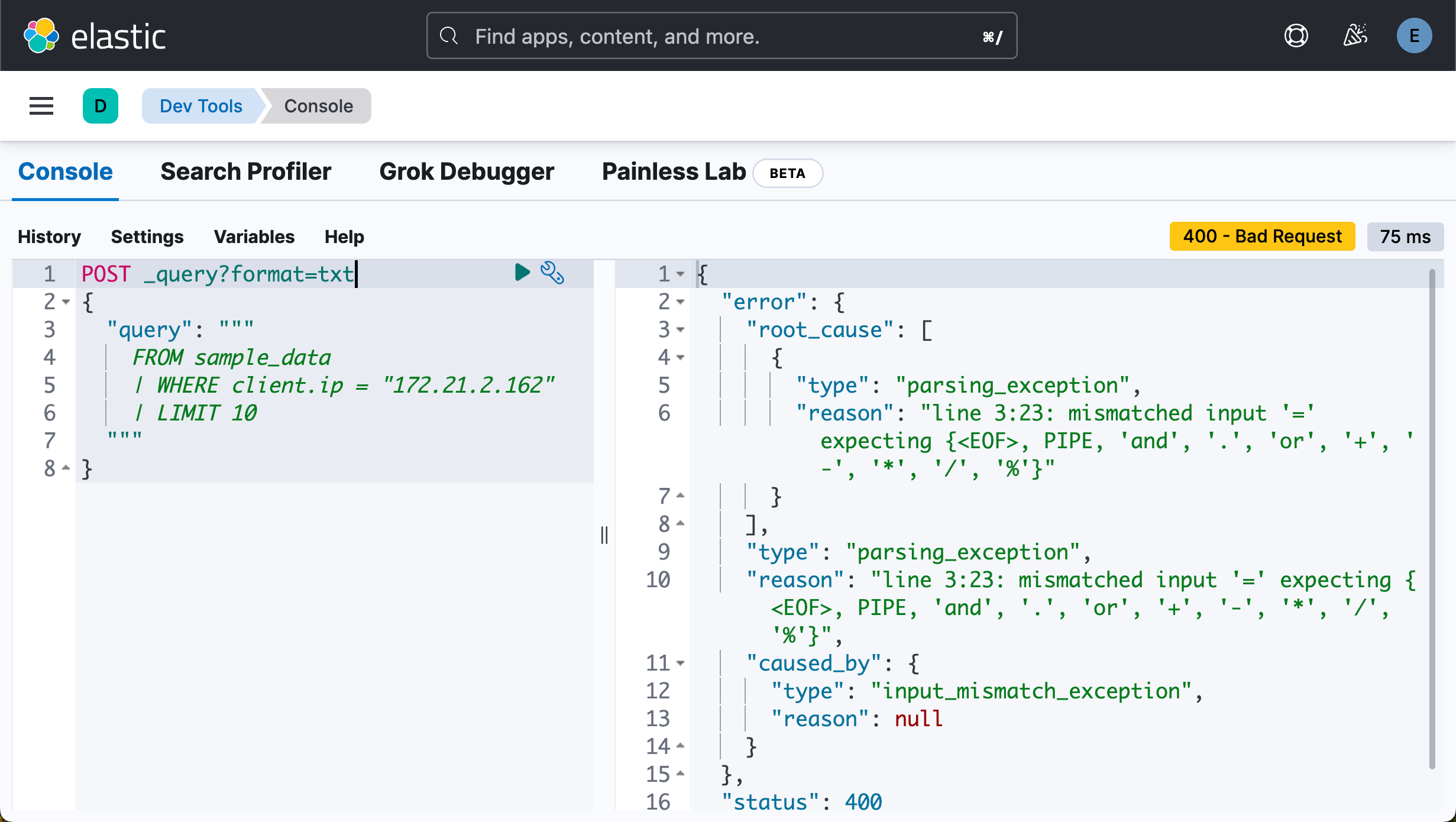
在上面 “=” 是一个赋值操作符。两个数据的类型不一样，不能赋值。

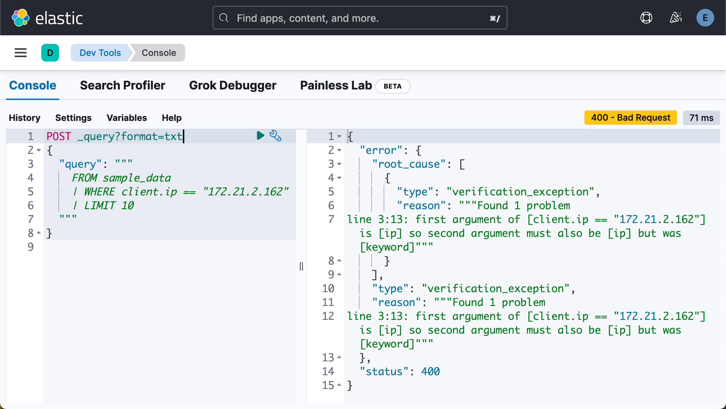
POST _query?format=txt
{
  "query": """
    FROM sample_data
    | WHERE client.ip == "172.21.2.162"
    | LIMIT 10
  """
}

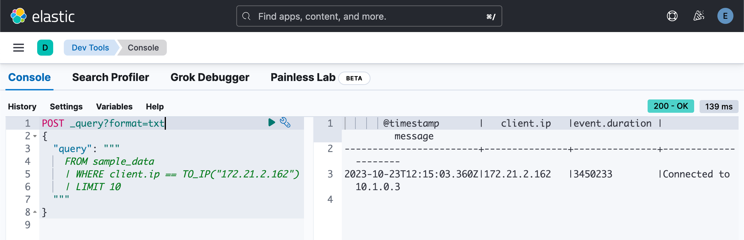
POST _query?format=txt
{
  "query": """
    FROM sample_data
    | WHERE client.ip == TO_IP("172.21.2.162")
    | LIMIT 10
  """
}

我们可以通过类型转换来得到相同的数据类型：

你也可以做如下的查询：

POST _query?format=txt
{
  "query": """
    FROM sample_data
    | WHERE TO_STRING(client.ip) == "172.21.2.162"
    | LIMIT 10
  """
}

POST _query?format=txt
{
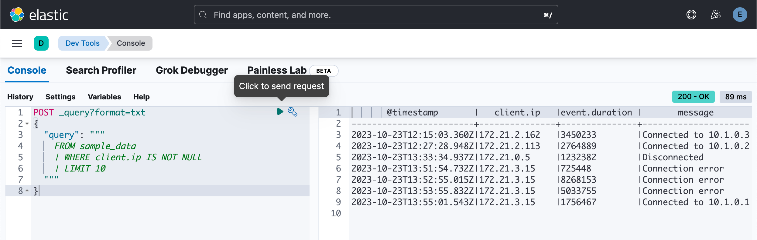
  "query": """
    FROM sample_data
    | WHERE client.ip IS NOT NULL
    | LIMIT 10
  """
}

我们可以看到和如下查询的区别：

POST /_query?format=csv
{
  "query": """
    FROM sample_data
    | sort @timestamp desc
    | LIMIT 5
  """
}

在上面，我们交互了 sort 及 LIMIT 的顺序，我们可以看到查询结果的变化：

上述命令类似于 DSL：

GET sample_data/_search
{
  "size": 5,
  "sort": [
    {
      "@timestamp": {
        "order": "desc"
      }
    }
  ]
}

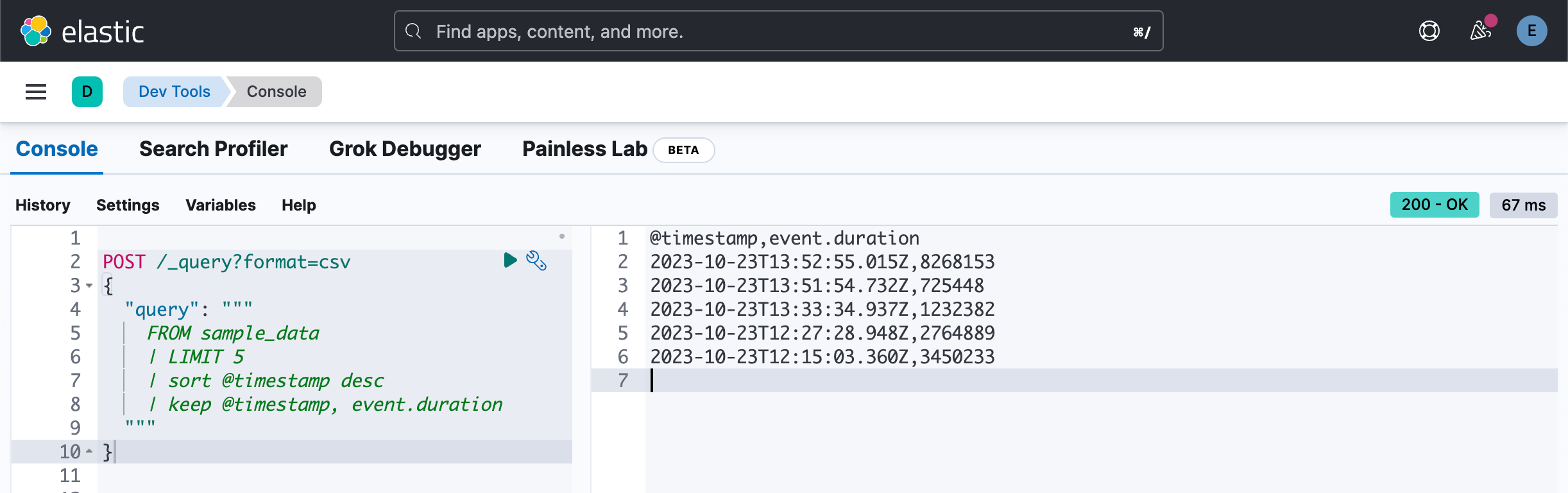
我们可以使用 keep 来返回我们想要的字段：

POST /_query?format=csv
{
  "query": """
    FROM sample_data
    | LIMIT 5
    | sort @timestamp desc
    | keep @timestamp, event.duration
  """
}

GET sample_data/_search?size=5
{
  "_source": ["@timestamp", "event.duration"], 
  "sort": [
    {
      "@timestamp": {
        "order": "desc"
      }
    }
  ]
}

或者：

GET sample_data/_search?size=5
{
  "_source": false, 
  "sort": [
    {
      "@timestamp": {
        "order": "desc"
      }
    }
  ],
  "fields": [
    "@timestamp",
    "event.duration"
  ]
}

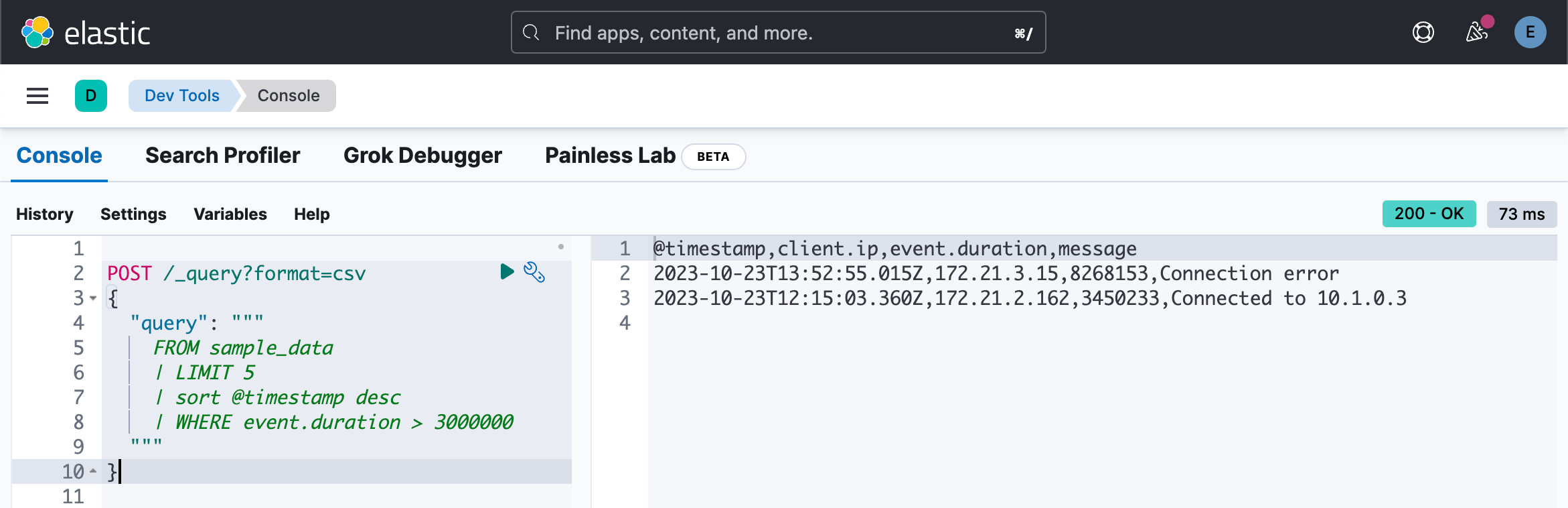
查询数据

我们可以针对数据来进行查询：

POST /_query?format=csv
{
  "query": """
    FROM sample_data
    | LIMIT 5
    | sort @timestamp desc
    | WHERE event.duration > 3000000
  """
}

我们甚至可以含有多个 WHERE 查询：

POST /_query?format=csv
{
  "query": """
    FROM sample_data
    | LIMIT 5
    | sort @timestamp desc
    | WHERE event.duration > 3000000
    | WHERE message LIKE "Connection *"
  """
}

这个类似于 DSL 的如下查询：

GET sample_data/_search
{
  "size": 5,
  "query": {
    "bool": {
      "must": [
        {
          "wildcard": {
            "message": {
              "value": "Connection *"
            }
          }
        }
      ],
      "filter": [
        {
          "range": {
            "event.duration": {
              "gt": 3000000
            }
          }
        }
      ]
    }
  }
}

确切地说和下面的类似：

POST /_query?format=csv
{
  "query": """
    FROM sample_data
    | sort @timestamp desc
    | WHERE event.duration > 3000000
    | WHERE message LIKE "Connection *"
    | LIMIT 5
  """
}

我们可以也可以使用 DROP 来删除我们不需要的列，比如 client.ip：

POST /_query?format=csv
{
  "query": """
    FROM sample_data
    | LIMIT 5
    | sort @timestamp desc
    | WHERE event.duration > 3000000
    | WHERE message LIKE "Connection *"
    | DROP client.ip
  """
}

在上面，我们删除了 client.ip 这个字段。这个和下面的 DSL 类似：

GET sample_data/_search
{
  "size": 5,
  "_source": {
    "excludes": [
      "client.ip"
    ]
  },
  "query": {
    "bool": {
      "must": [
        {
          "wildcard": {
            "message": {
              "value": "Connection *"
            }
          }
        }
      ],
      "filter": [
        {
          "range": {
            "event.duration": {
              "gt": 3000000
            }
          }
        }
      ]
    }
  }
}

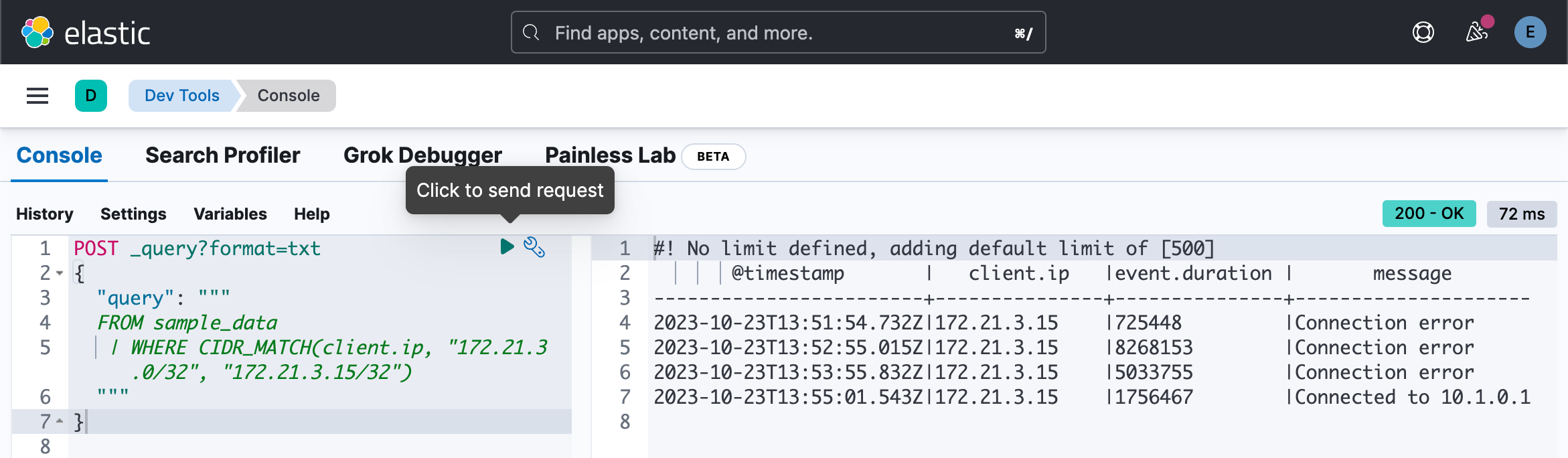
针对 ip 进行搜索：

POST _query?format=txt
{
  "query": """
  FROM sample_data
   | WHERE CIDR_MATCH(client.ip, "172.21.3.0/32", "172.21.3.15/32")
  """
}

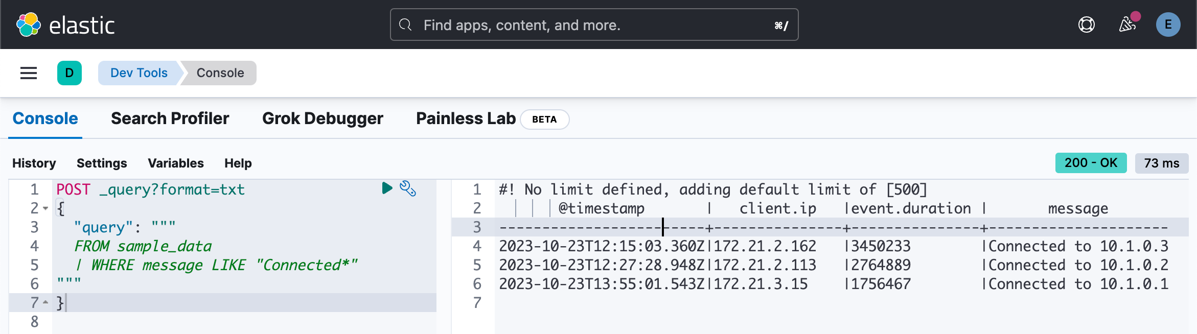
文本搜索

我们可以使用 ES|QL 针对文字进行搜索。由于目前的一些限制，它把 text 当做是 keyword。具体请详细查看文章 “Elasticsearch：ES|QL 的限制”。在目前的版中中，我们仅可以针对 keyword 进行搜索：

POST _query?format=txt
{
  "query": """
  FROM sample_data
  | WHERE message LIKE "Connected*"
"""
}

但是如下的查询是没有任何结果的：

POST _query?format=txt
{
  "query": """
  FROM sample_data
  | WHERE message LIKE "Connected"
"""
}

或：

POST _query?format=txt
{
  "query": """
  FROM sample_data
  | WHERE message LIKE "connected*"
"""
}

我们可以使用如下的查询返回结果：

POST _query?format=txt
{
  "query": """
  FROM sample_data
  | WHERE message RLIKE "[cC]onnected.*"
  """
}

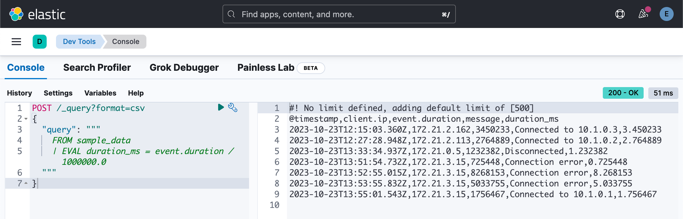
计算值

使用 EVAL 命令将包含计算值的列追加到表中。例如，以下查询附加一个 duration_ms 列。该列中的值是通过将 event.duration 除以 1,000,000 计算得出的。换句话说： event.duration 从纳秒转换为毫秒。

POST /_query?format=csv
{
  "query": """
    FROM sample_data
    | EVAL duration_ms = event.duration / 1000000.0
  """
}

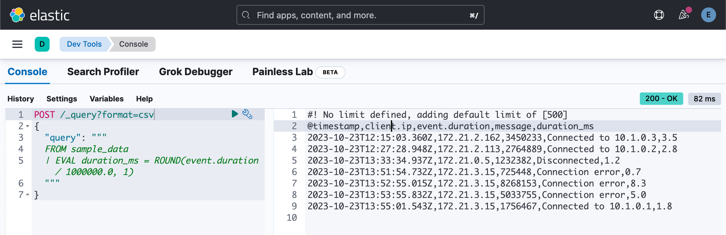
EVAL 支持多种 functions。例如，要将数字四舍五入为最接近指定位数的数字，请使用 ROUND 函数：

POST /_query?format=csv
{
  "query": """
  FROM sample_data
  | EVAL duration_ms = ROUND(event.duration / 1000000.0, 1)
  """
}

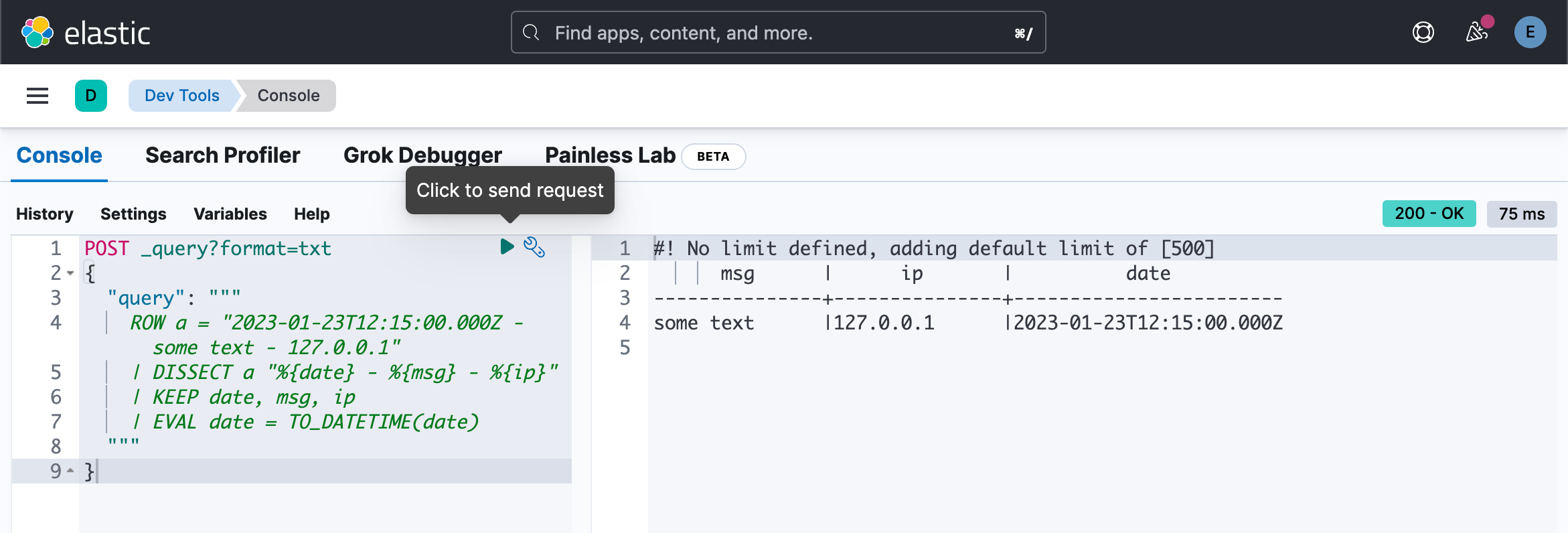
POST _query?format=txt
{
  "query": """
    ROW a = "2023-01-23T12:15:00.000Z - some text - 127.0.0.1"
    | DISSECT a "%{date} - %{msg} - %{ip}"
    | KEEP date, msg, ip
    | EVAL date = TO_DATETIME(date)
  """
}

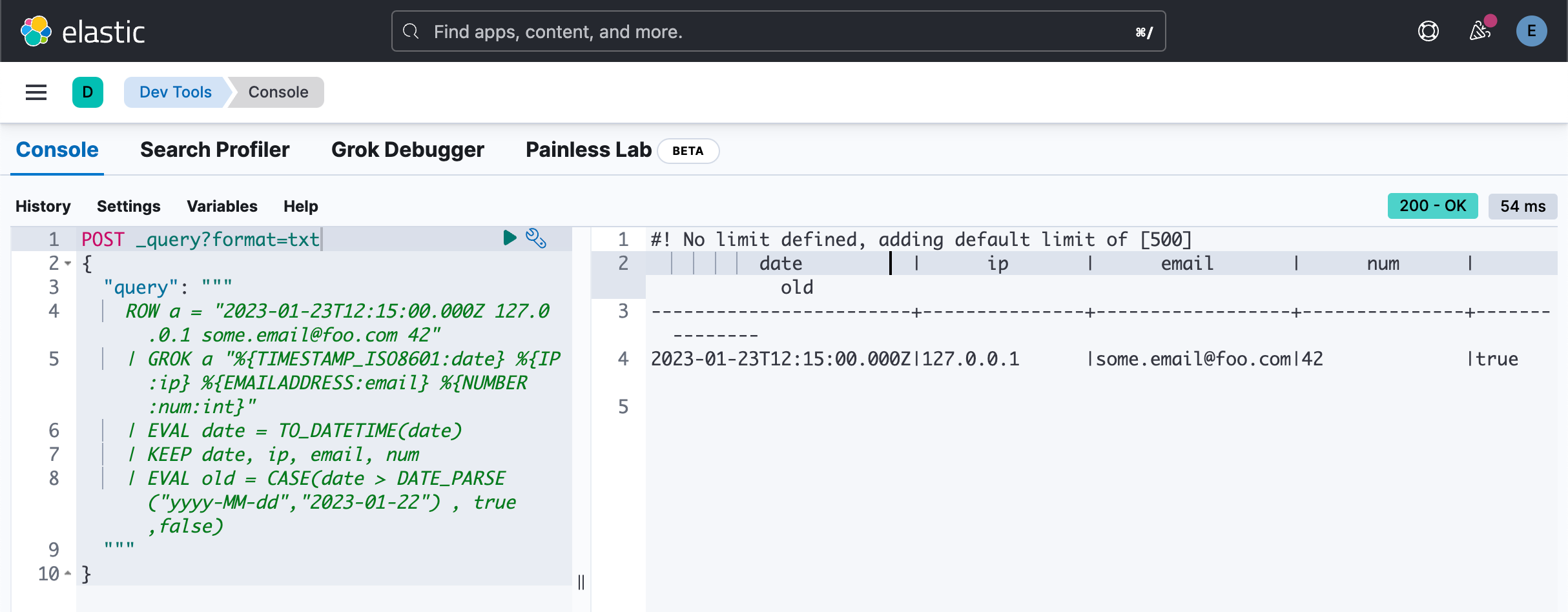
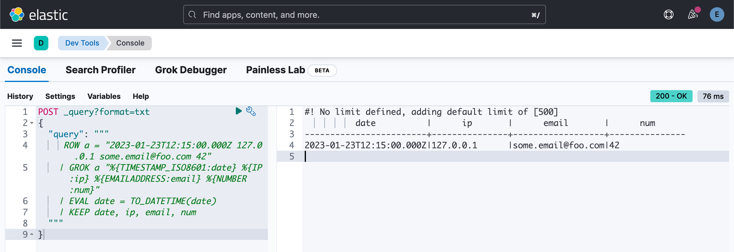
我们还可以比较时间：

POST _query?format=txt
{
  "query": """
    ROW a = "2023-01-23T12:15:00.000Z 127.0.0.1 some.email@foo.com 42"
    | GROK a "%{TIMESTAMP_ISO8601:date} %{IP:ip} %{EMAILADDRESS:email} %{NUMBER:num:int}"
    | EVAL date = TO_DATETIME(date)
    | KEEP date, ip, email, num
    | EVAL old = CASE(date > DATE_PARSE("yyyy-MM-dd","2023-01-22") , true,false)
  """
}

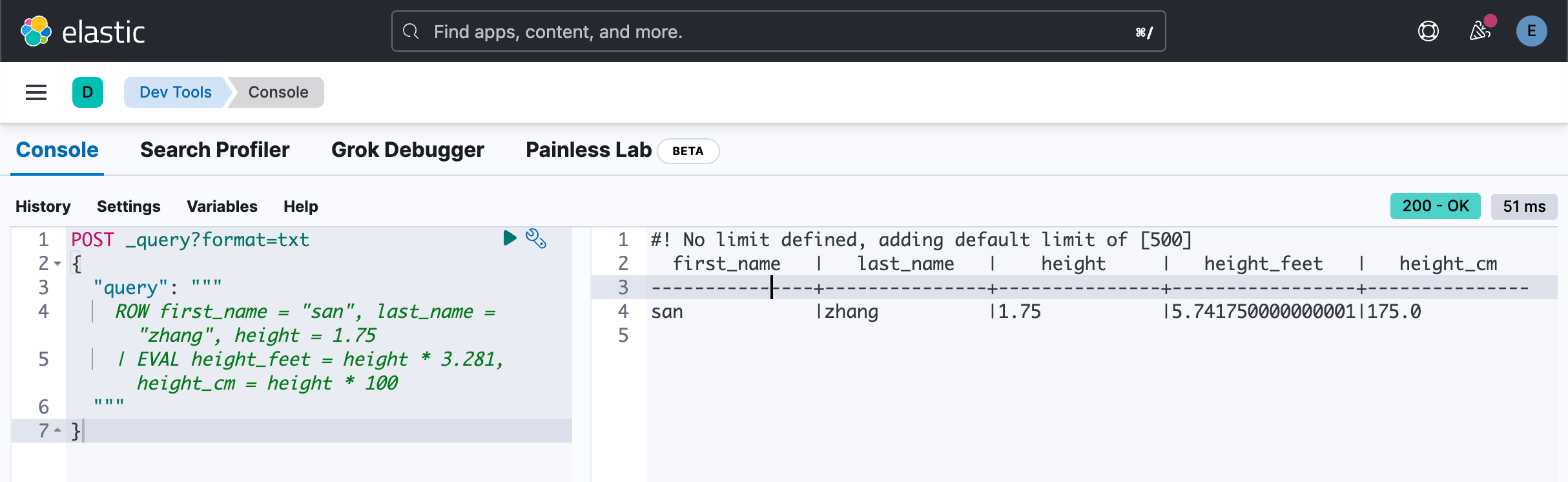
POST _query?format=txt
{
  "query": """
    ROW first_name = "san", last_name = "zhang", height = 1.75
    | EVAL height_feet = height * 3.281, height_cm = height * 100
  """
}

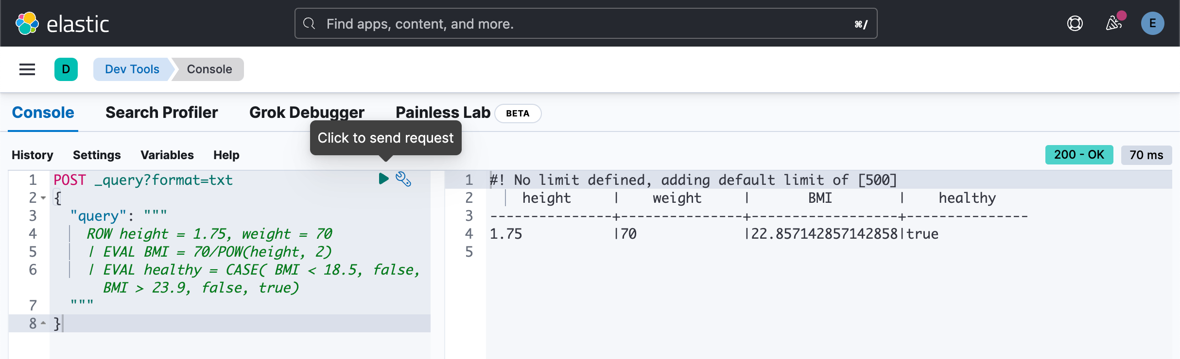
POST _query?format=txt
{
  "query": """
    ROW height = 1.75, weight = 70
    | EVAL BMI = 70/POW(height, 2)
    | EVAL healthy = CASE( BMI < 18.5, false, BMI > 23.9, false, true)
  """
}

使用 DISSECT

你的数据可能包含非结构化字符串，你希望将其结构化以便更轻松地分析数据。例如，示例数据包含如下日志消息：

"Connected to 10.1.0.3"
通过从这些消息中提取 IP 地址，你可以确定哪个 IP 接受了最多的客户端连接。

要在查询时构建非结构化字符串，你可以使用 ES|QL DISSECT 和 GROK 命令。 DISSECT 的工作原理是使用基于分隔符的模式分解字符串。 GROK 的工作原理类似，但使用正则表达式。这使得 GROK 更强大，但通常也更慢。

在这种情况下，不需要正则表达式，因为 message 很简单：“Connected to ”，后跟服务器 IP。要匹配此字符串，你可以使用以下 DISSECT 命令：

POST _query/?format=csv
{
  "query": """
  FROM sample_data
    | DISSECT message "Connected to %{server.ip}"
  """
}

这会将 server.ip 列添加到具有与此模式匹配的消息的那些行。对于其他行，server.ip 的值为空。

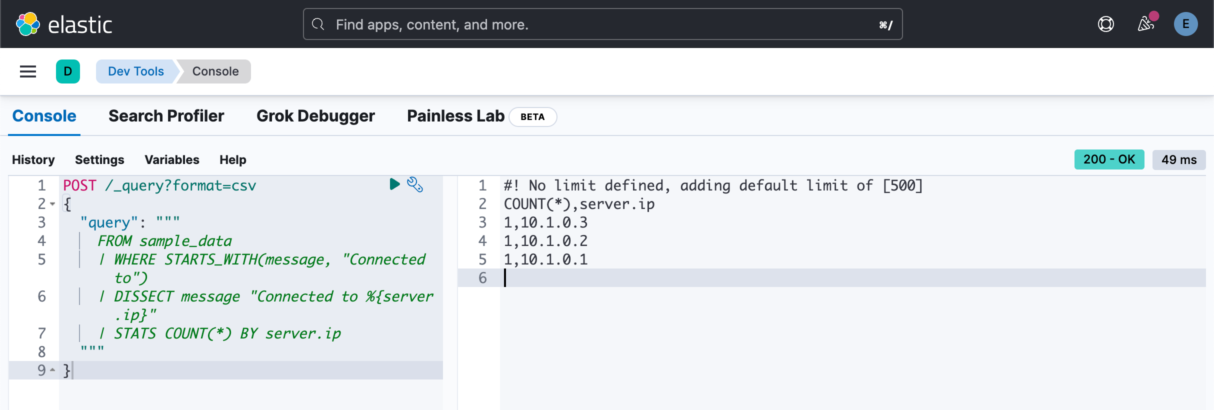
你可以在后续命令中使用 DISSECT 命令添加的新 server.ip 列。例如，要确定每个服务器已接受多少个连接：

POST /_query?format=csv
{
  "query": """
    FROM sample_data
    | WHERE STARTS_WITH(message, "Connected to")
    | DISSECT message "Connected to %{server.ip}"
    | STATS COUNT(*) BY server.ip
  """
}

使用 GROK

以下示例解析包含时间戳、IP 地址、电子邮件地址和数字的字符串：

POST _query?format=txt
{
  "query": """
     ROW a = "2023-01-23T12:15:00.000Z 127.0.0.1 some.email@foo.com 42"
    | GROK a "%{TIMESTAMP_ISO8601:date} %{IP:ip} %{EMAILADDRESS:email} %{NUMBER:num}"
    | EVAL date = TO_DATETIME(date)
    | KEEP date, ip, email, num
  """
}

聚合

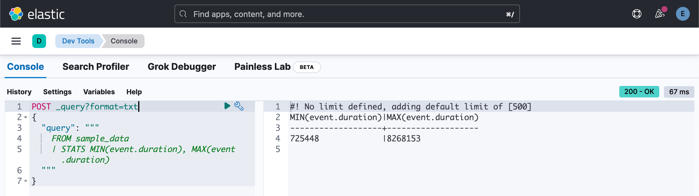
找出 event.duration 的最大值及最小值：

POST _query?format=txt
{
  "query": """
    FROM sample_data
    | STATS MIN(event.duration), MAX(event.duration)
  """
}

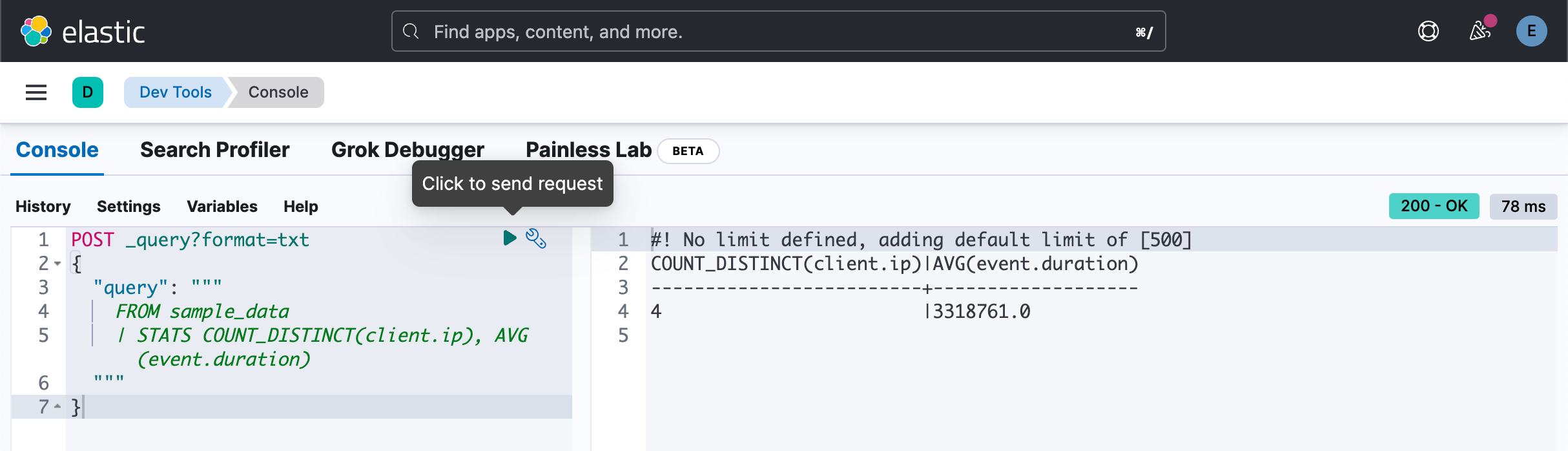
我们找出有多少个 client.ip，以及 event.duration 的平均值：

POST _query?format=txt
{
  "query": """
    FROM sample_data
    | STATS COUNT_DISTINCT(client.ip), AVG(event.duration)
  """
}

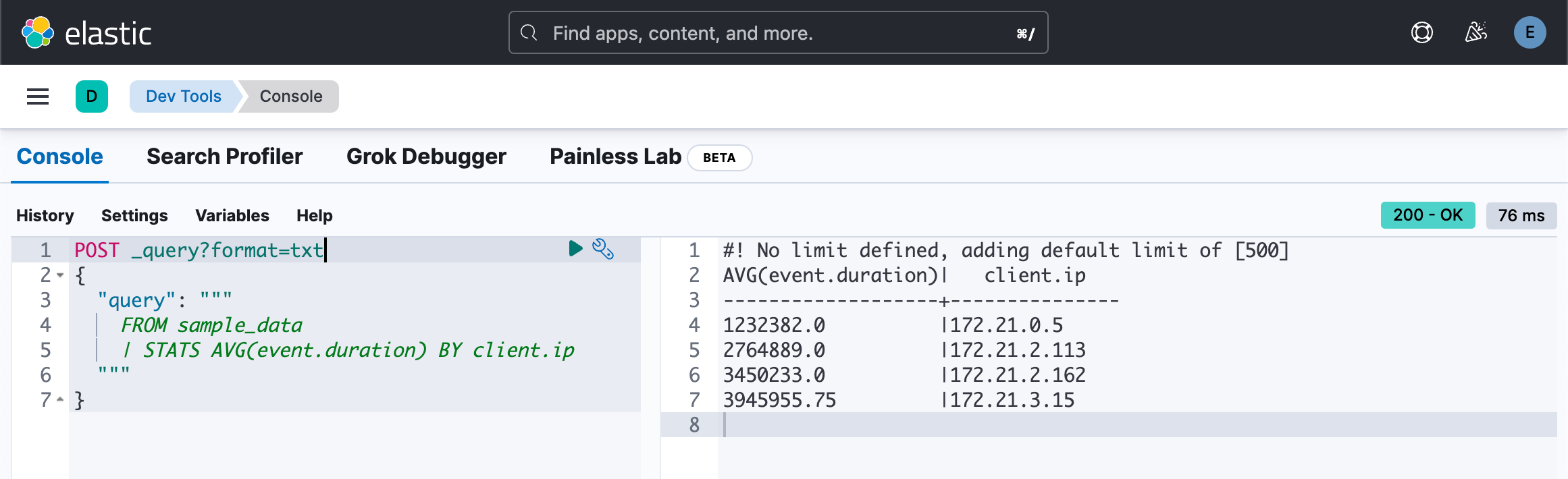
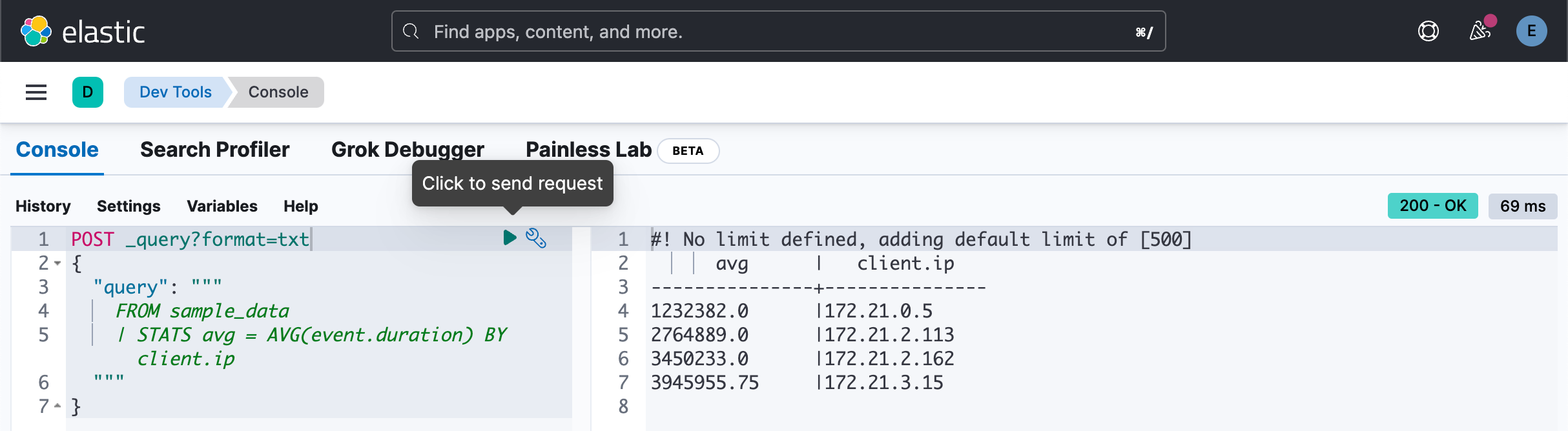
我们想知道每个 client.ip 的平均 event.duration 值：

POST _query?format=txt
{
  "query": """
    FROM sample_data
    | STATS AVG(event.duration) BY client.ip
  """
}

POST _query?format=txt
{
  "query": """
    FROM sample_data
    | STATS AVG(event.duration), COUNT(*) BY client.ip
    | SORT COUNT(*)
  """
}

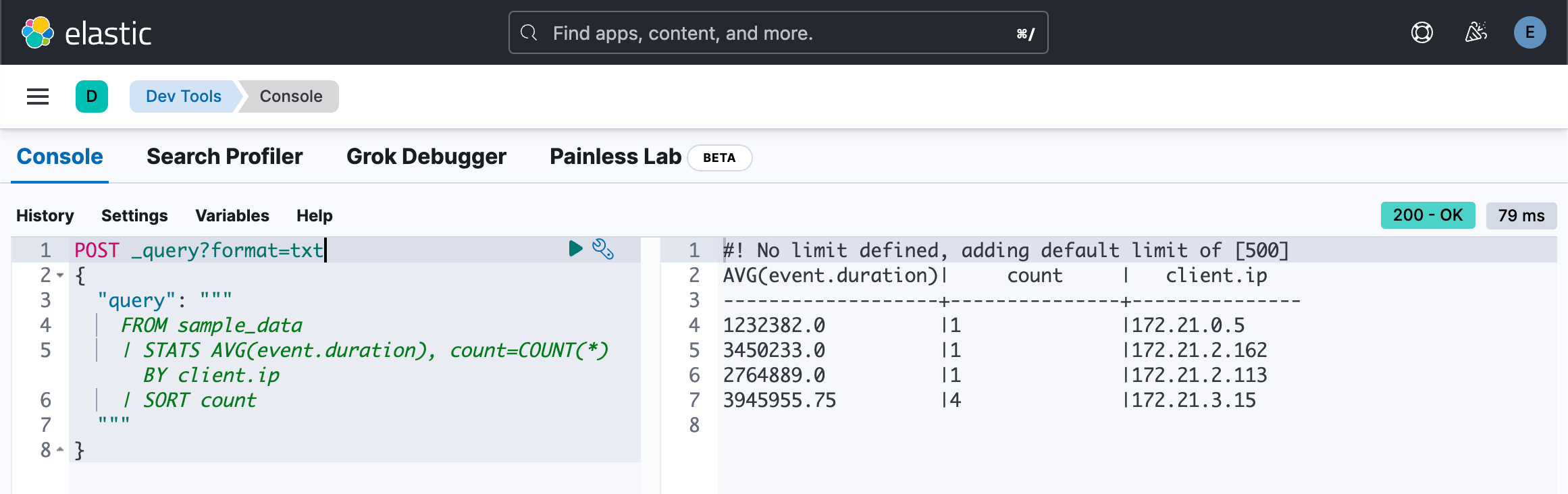
上面的查询会失败。原因是 COUNT(*) 不是一个变量。我们可以使用如下的方法：

POST _query?format=txt
{
  "query": """
    FROM sample_data
    | STATS AVG(event.duration), count=COUNT(*) BY client.ip
    | SORT count
  """
}

或者：

POST _query?format=txt
{
  "query": """
    FROM sample_data
    | STATS AVG(event.duration), COUNT(*) BY client.ip
    | SORT `COUNT(*)`
  """
}

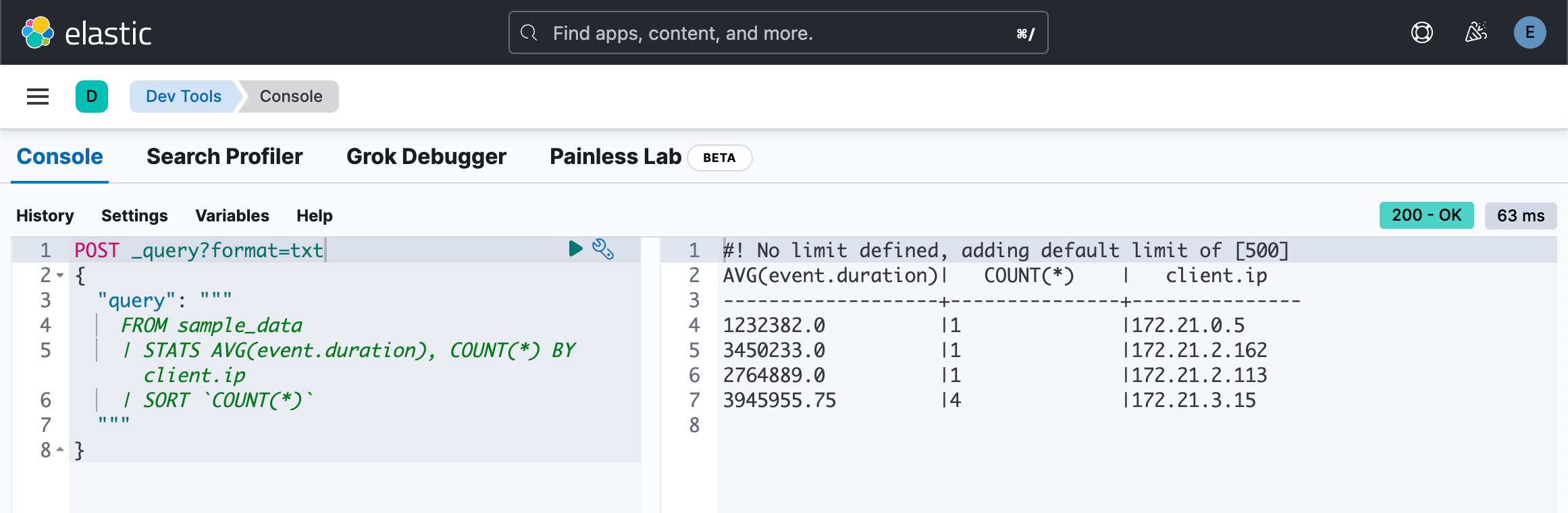
请注意上面的符号是 ` 而不是 '。

如果我们把上面的 COUNT 换成小写的 count：

POST _query?format=txt
{
  "query": """
    FROM sample_data
    | STATS AVG(event.duration), COUNT(*) BY client.ip
    | SORT `count(*)`
  """
}

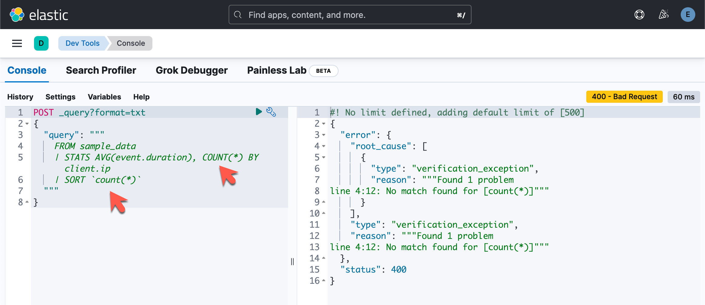
原因是上面的两个 counts：一个是大写的，一个是小写的。它们不匹配。必须同时是大写，或者同时是小写。

POST _query?format=txt
{
  "query": """
    FROM sample_data
    | STATS avg = AVG(event.duration) BY client.ip
  """
}

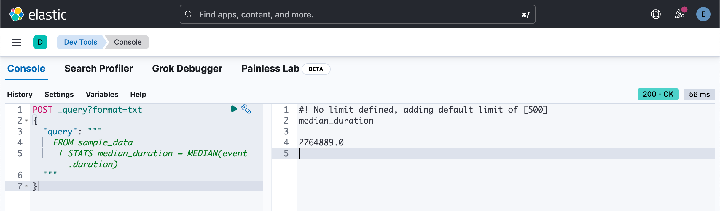
POST _query?format=txt
{
  "query": """
    FROM sample_data
     | STATS median_duration = MEDIAN(event.duration)
  """
}

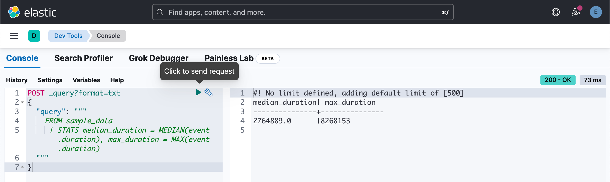
POST _query?format=txt
{
  "query": """
    FROM sample_data
     | STATS median_duration = MEDIAN(event.duration), max_duration = MAX(event.duration)
  """
}

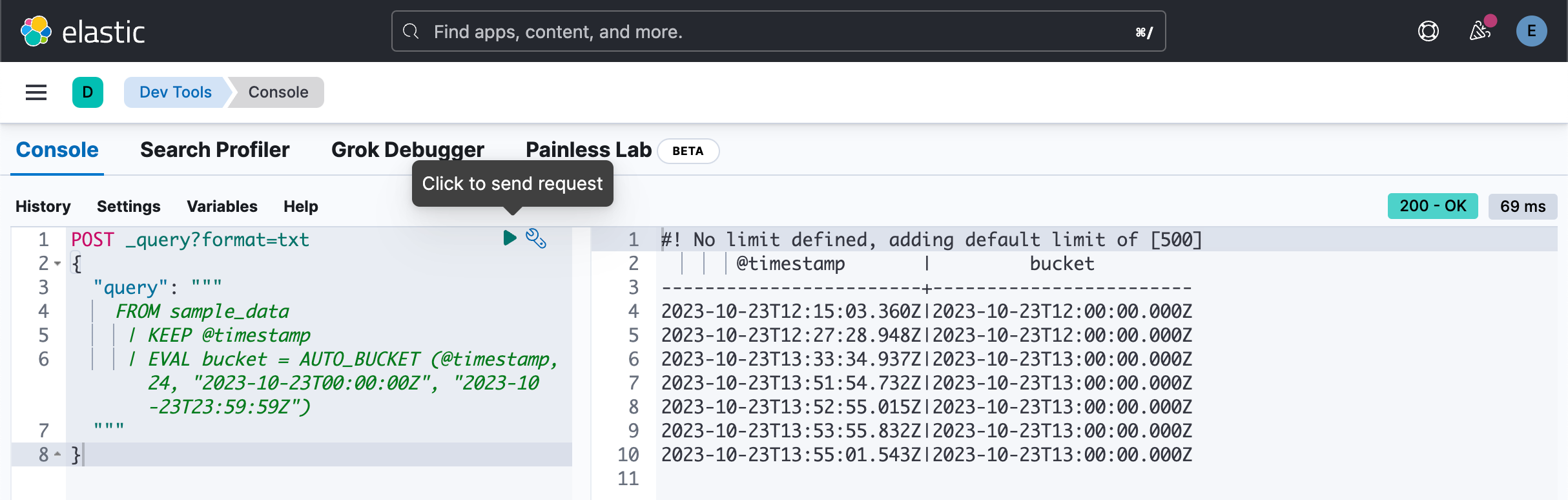
创建直方图

为了跟踪一段时间内的统计数据，ES|QL 允许你使用 AUTO_BUCKET 函数创建直方图。 AUTO_BUCKET 创建人性化的存储桶大小，并为每行返回一个与该行所属的结果存储桶相对应的值。

例如，要为 10 月 23 日的数据创建每小时存储桶：

POST _query?format=txt
{
  "query": """
    FROM sample_data
     | KEEP @timestamp
     | EVAL bucket = AUTO_BUCKET (@timestamp, 24, "2023-10-23T00:00:00Z", "2023-10-23T23:59:59Z")
  """
}

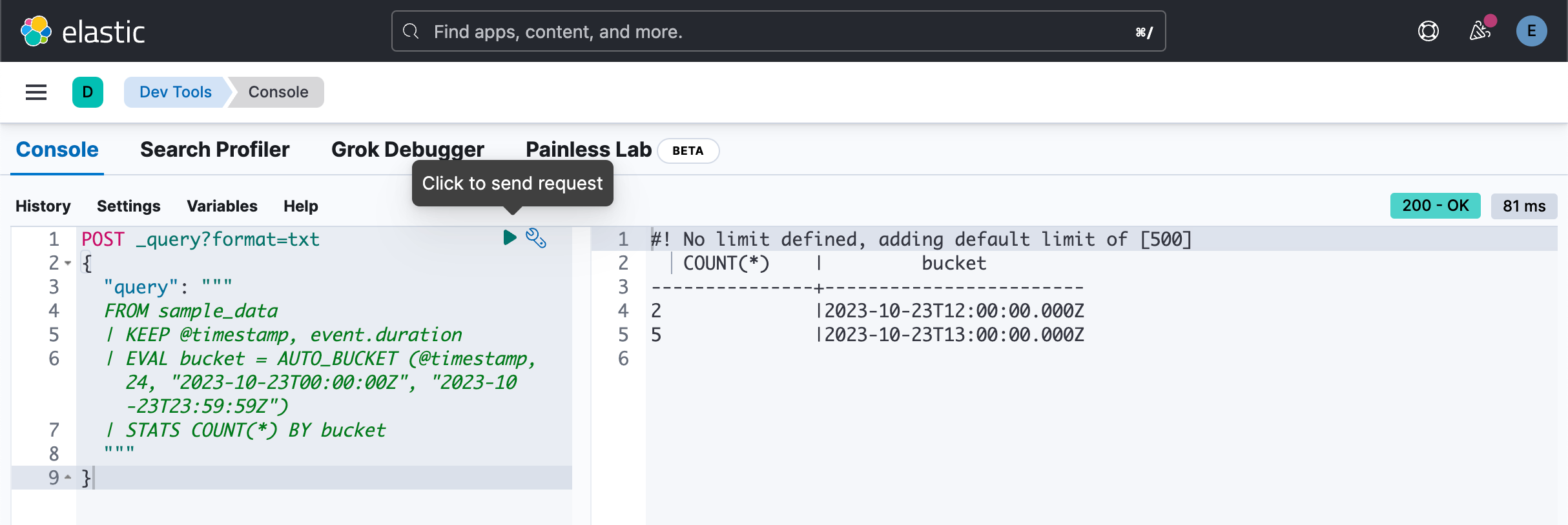
将 AUTO_BUCKET 与 STATS ... BY 结合起来创建直方图。例如，要计算每小时的事件数：

POST _query?format=txt
{
  "query": """
  FROM sample_data
  | KEEP @timestamp, event.duration
  | EVAL bucket = AUTO_BUCKET (@timestamp, 24, "2023-10-23T00:00:00Z", "2023-10-23T23:59:59Z")
  | STATS COUNT(*) BY bucket
  """
}

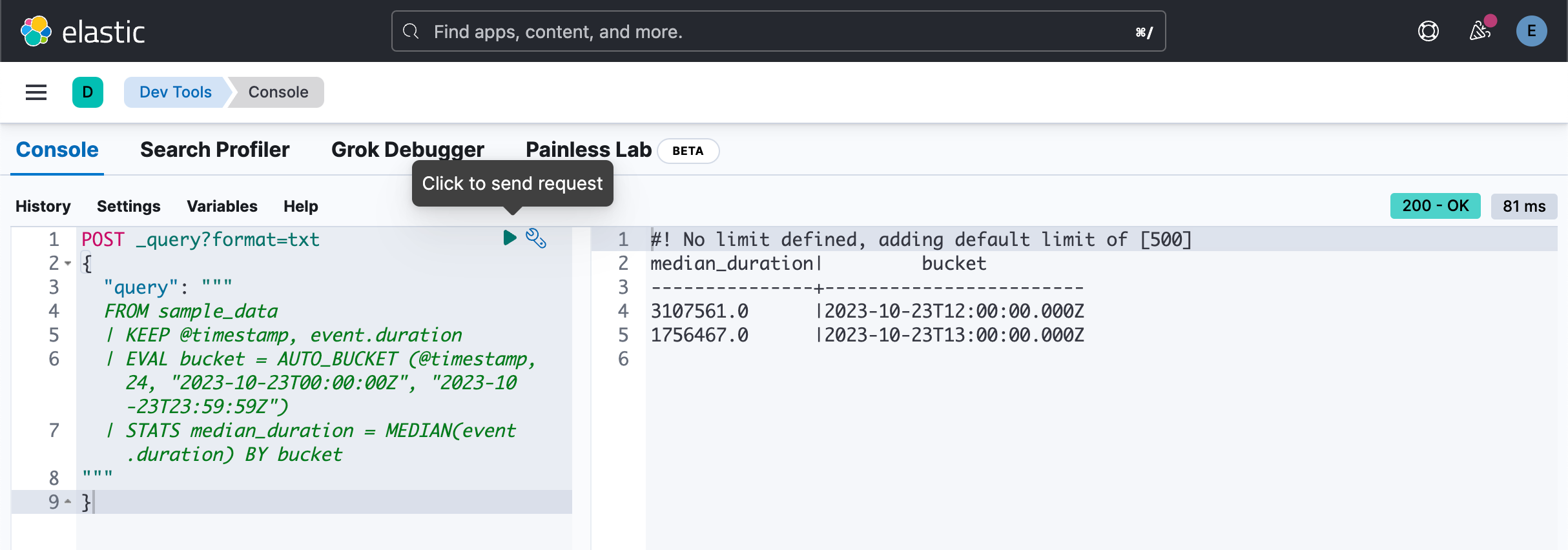
每个小时的中位数统计：

POST _query?format=txt
{
  "query": """
  FROM sample_data
  | KEEP @timestamp, event.duration
  | EVAL bucket = AUTO_BUCKET (@timestamp, 24, "2023-10-23T00:00:00Z", "2023-10-23T23:59:59Z")
  | STATS median_duration = MEDIAN(event.duration) BY bucket
"""
}

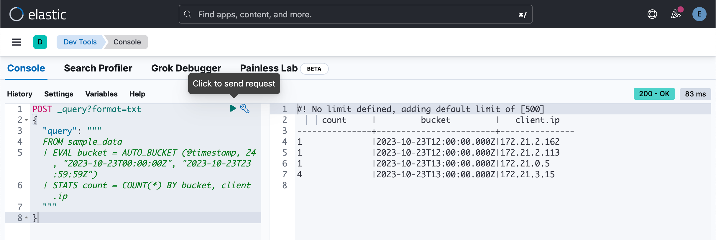
我们更进一步对每个桶做细分，比如更进一步根据每个 client.ip 进行统计：

POST _query?format=txt
{
  "query": """
  FROM sample_data
  | EVAL bucket = AUTO_BUCKET (@timestamp, 24, "2023-10-23T00:00:00Z", "2023-10-23T23:59:59Z")
  | STATS count = COUNT(*) BY bucket, client.ip
  """
}

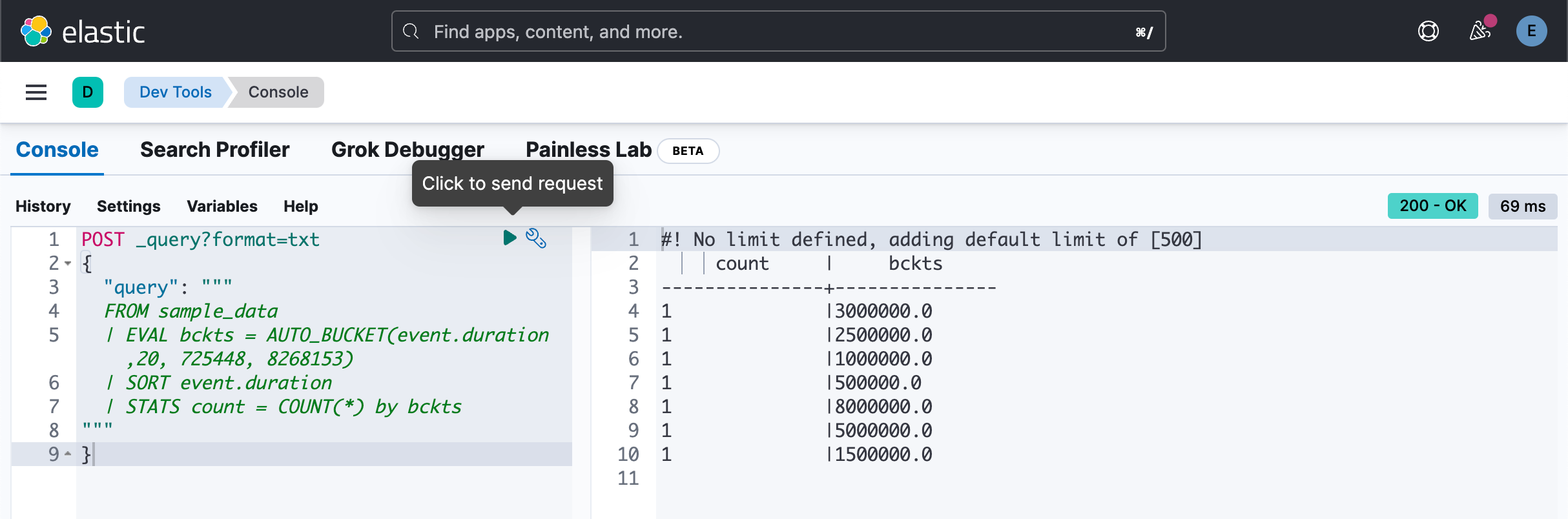
针对数字字段的桶分析

auto_bucket 还可以对数字字段进行操作，如下所示：

POST _query?format=txt
{
  "query": """
  FROM sample_data
  | EVAL bckts = AUTO_BUCKET(event.duration,20, 725448, 8268153)
  | SORT event.duration
  | STATS count = COUNT(*) by bckts
"""
}

丰富数据

ES|QL 使你能够使用 ENRICH 命令使用 Elasticsearch 中索引的数据来丰富表。

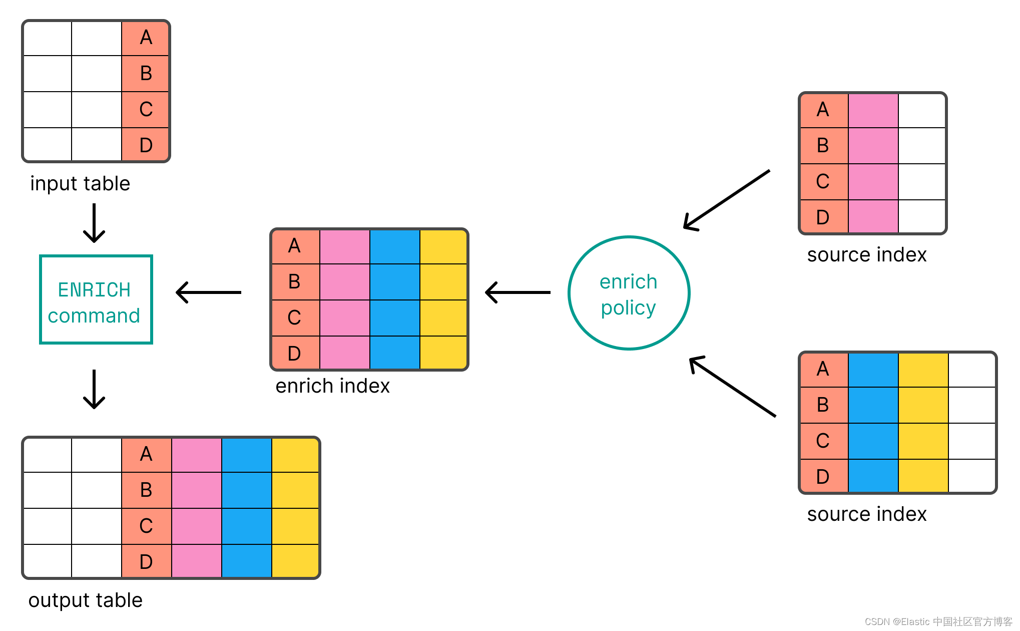
在使用 ENRICH 之前，你首先需要 create 并 execute 你的 enrich policy。以下请求创建并执行将 IP 地址链接到环境（“Development”、“QA” 或 “Production”）的策略：

PUT clientips
{
  "mappings": {
    "properties": {
      "client.ip": {
        "type": "keyword"
      },
      "env": {
        "type": "keyword"
      }
    }
  }
}

PUT clientips/_bulk
{ "index" : {}}
{ "client.ip": "172.21.0.5", "env": "Development", "location": "loc1" }
{ "index" : {}}
{ "client.ip": "172.21.2.113", "env": "QA", "location": "loc2" }
{ "index" : {}}
{ "client.ip": "172.21.2.162", "env": "QA", "location": "loc3" }
{ "index" : {}}
{ "client.ip": "172.21.3.15", "env": "Production", "location":"loc4" }
{ "index" : {}}
{ "client.ip": "172.21.3.16", "env": "Production", "location": "loc5" }

PUT /_enrich/policy/clientip_policy
{
  "match": {
    "indices": "clientips",
    "match_field": "client.ip",
    "enrich_fields": ["env", "location"]
  }
}

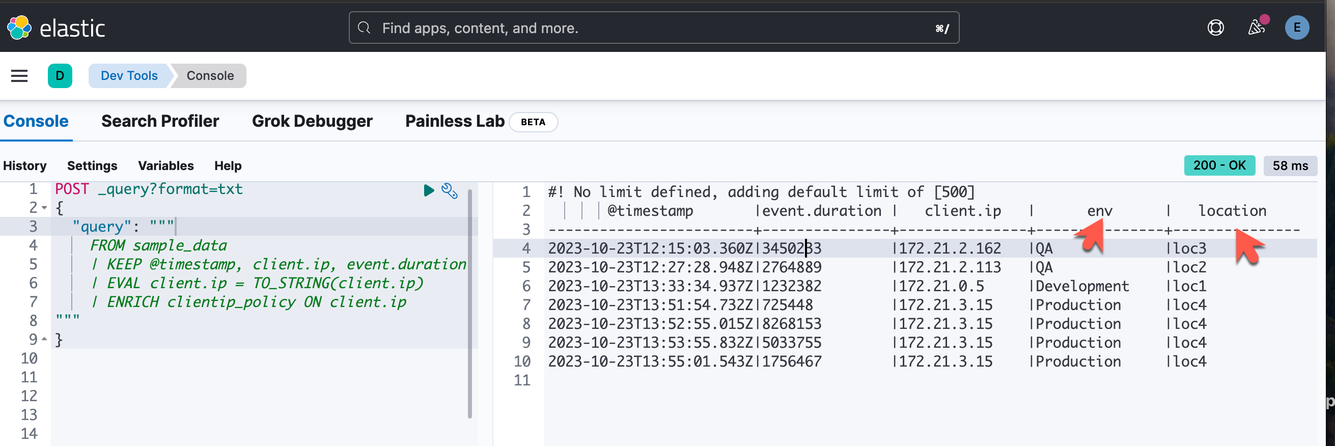
PUT /_enrich/policy/clientip_policy/_execute

创建并执行策略后，你可以将其与 ENRICH 命令一起使用：

POST _query?format=txt
{
  "query": """
    FROM sample_data
    | KEEP @timestamp, client.ip, event.duration
    | EVAL client.ip = TO_STRING(client.ip)
    | ENRICH clientip_policy ON client.ip
"""
}

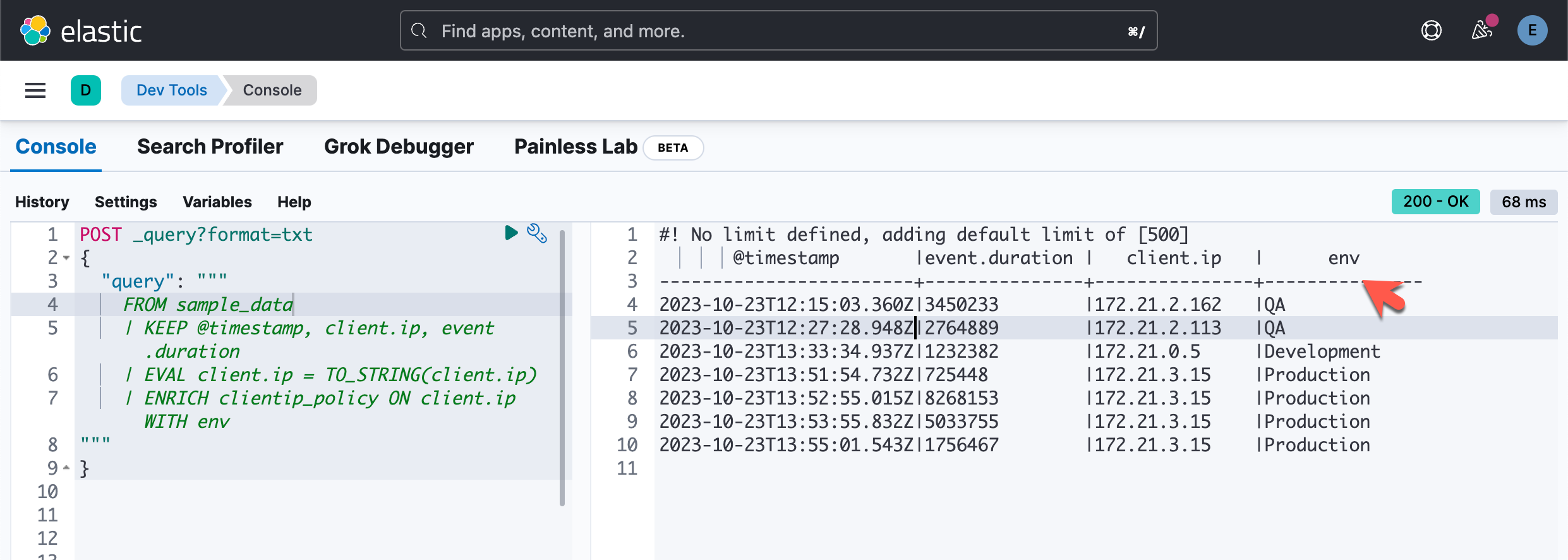
POST _query?format=txt
{
  "query": """
    FROM sample_data
    | KEEP @timestamp, client.ip, event.duration
    | EVAL client.ip = TO_STRING(client.ip)
    | ENRICH clientip_policy ON client.ip WITH env
"""
}

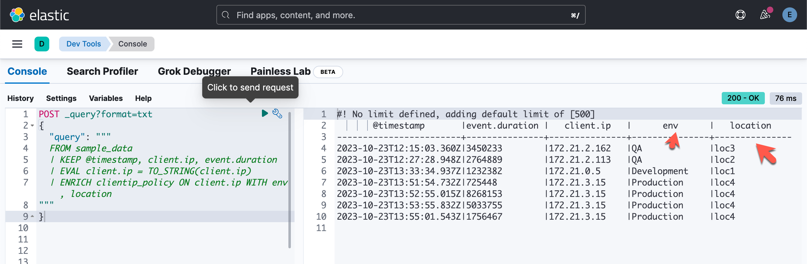
我们还可以添加其它定义在 clientip_policy 里的字段，比如：

POST _query?format=txt
{
  "query": """
  FROM sample_data
  | KEEP @timestamp, client.ip, event.duration
  | EVAL client.ip = TO_STRING(client.ip)
  | ENRICH clientip_policy ON client.ip WITH env, location
"""
}

在上面，我们添加了 location：

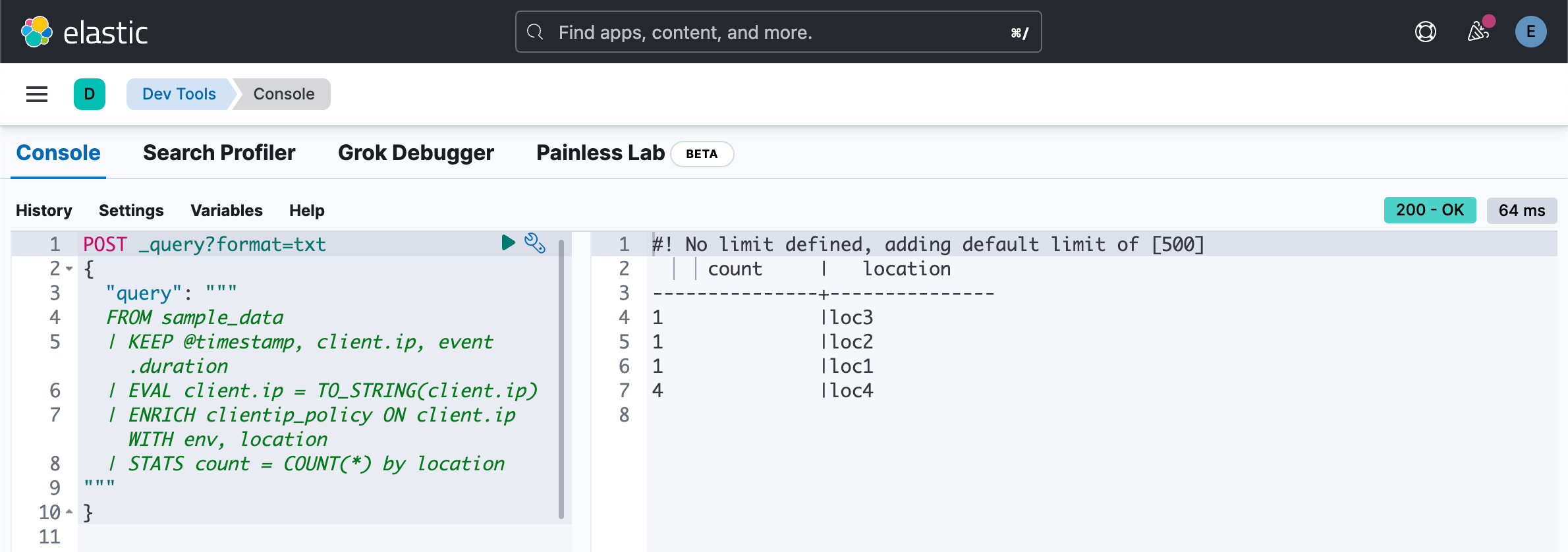
我们甚至可以针对这些被丰富的字段进行聚会：

POST _query?format=txt
{
  "query": """
  FROM sample_data
  | KEEP @timestamp, client.ip, event.duration
  | EVAL client.ip = TO_STRING(client.ip)
  | ENRICH clientip_policy ON client.ip WITH env, location
  | STATS count = COUNT(*) by location
"""
}

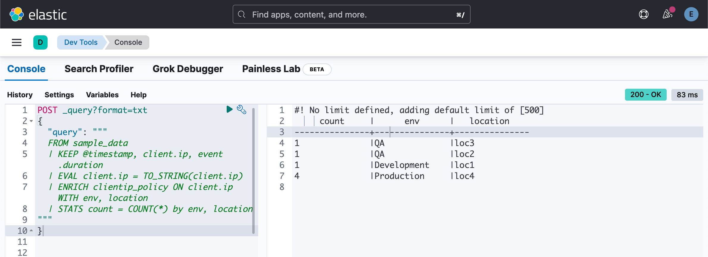
我还可以进行如下的统计：

POST _query?format=txt
{
  "query": """
  FROM sample_data
  | KEEP @timestamp, client.ip, event.duration
  | EVAL client.ip = TO_STRING(client.ip)
  | ENRICH clientip_policy ON client.ip WITH env, location
  | STATS count = COUNT(*) by env, location
"""
}

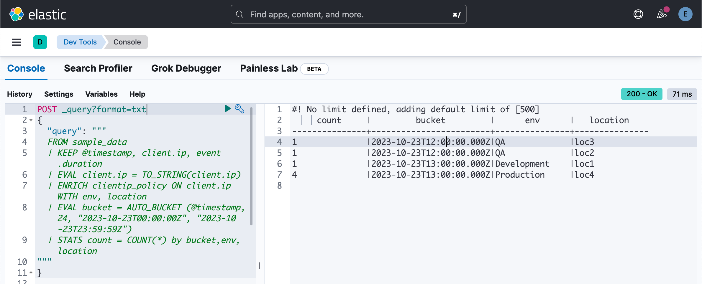
我们还可以进行如下的统计：

POST _query?format=txt
{
  "query": """
  FROM sample_data
  | KEEP @timestamp, client.ip, event.duration
  | EVAL client.ip = TO_STRING(client.ip)
  | ENRICH clientip_policy ON client.ip WITH env, location
  | EVAL bucket = AUTO_BUCKET (@timestamp, 24, "2023-10-23T00:00:00Z", "2023-10-23T23:59:59Z")
  | STATS count = COUNT(*) by bucket,env, location
"""
}

元数据运用

ES|QL 可以访问元数据字段。目前支持的有：

_index：文档所属的索引名称。该字段的类型为关键字。
_id：源文档的 ID。该字段的类型为关键字。
_version：源文档的版本。该字段的类型为 long。

要启用对这些字段的访问，需要为 FROM source 命令提供专用指令：

FROM index [METADATA _index, _id]

仅当数据源是索引时元数据字段才可用。因此，FROM 是唯一支持 METADATA 指令的源命令。比如，

POST _query?format=txt
{
  "query": """
    FROM sample_data [METADATA _index, _id]
    | LIMIT 3
  """
}

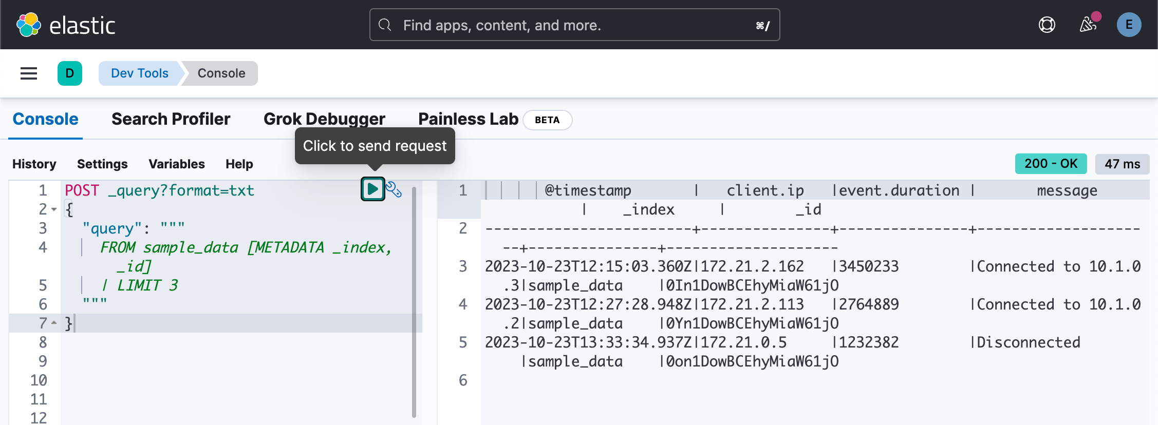
从上面的返回数据中，我们可以看到 _index 及 _id 返回索引名称 sample_data 及文档的 ID。

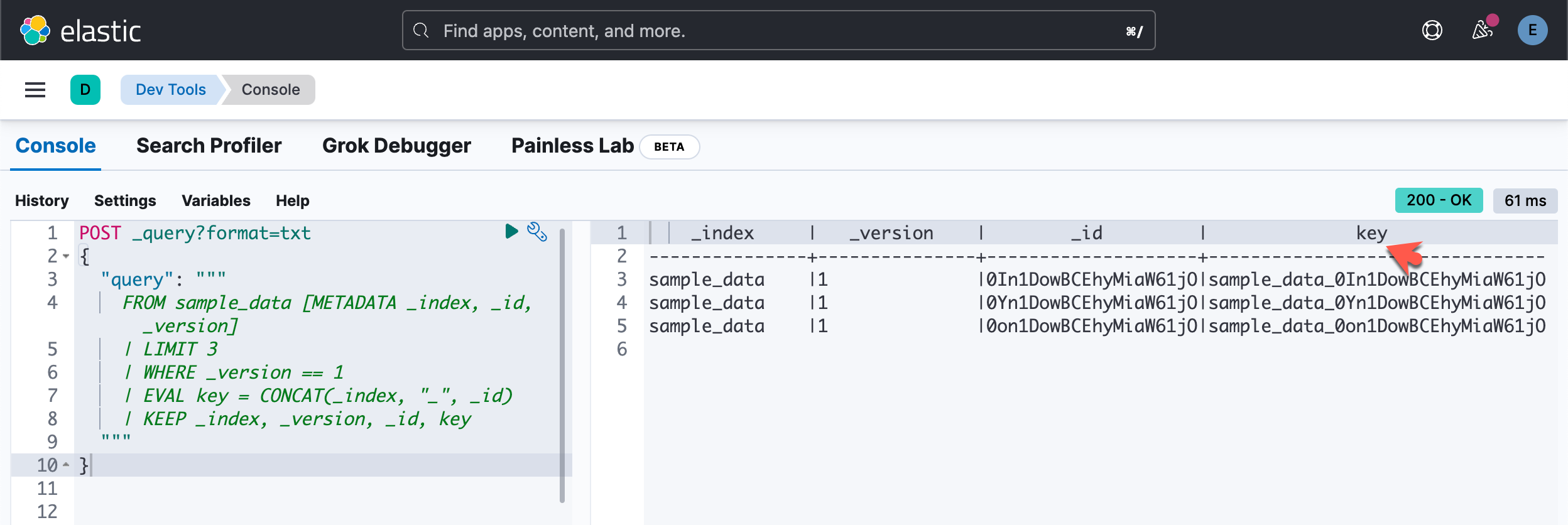
POST _query?format=txt
{
  "query": """
    FROM sample_data [METADATA _index, _id,  _version]
    | LIMIT 3
    | WHERE _version == 1
    | EVAL key = CONCAT(_index, "_", _id)
    | KEEP _index, _version, _id, key
  """
}

我们使用如下的命令来创建一个另外一个索引：

PUT sample_data/_bulk
{"index":{}}
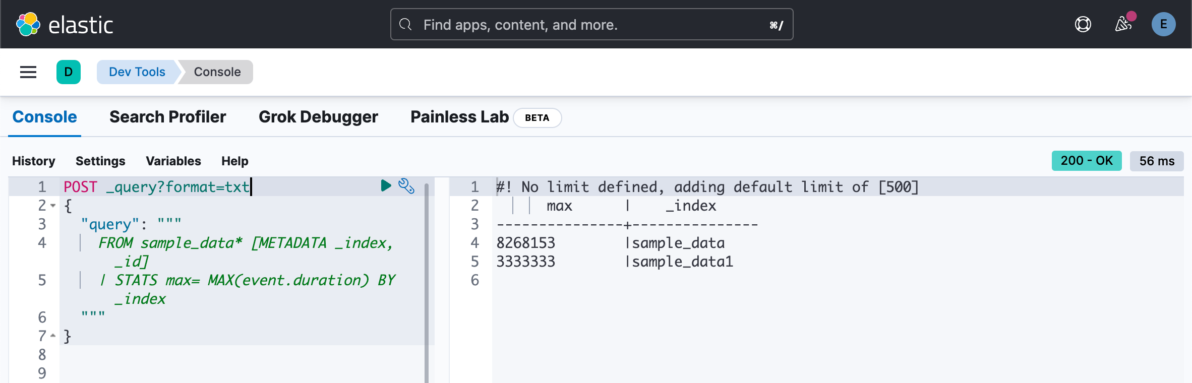
{"@timestamp":"2023-10-23T11:15:03.360Z","client.ip":"172.21.2.162","message":"Connected to 10.1.0.5","event.duration":3333333}

此外，与索引字段类似，一旦执行聚合，后续命令将无法再访问元数据字段，除非用作分组字段：

POST _query?format=txt
{
  "query": """
    FROM sample_data* [METADATA _index, _id]
    | STATS max= MAX(event.duration) BY _index
  """
}

ES|QL 多值字段

ES|QL 可以很好地读取多值字段。多值字段也就是在一个字段里有多个值。通常是以数组的形式出现。

POST /mv/_bulk?refresh
{"index":{}}
{"a":1,"b":[2,1]}
{"index":{}}
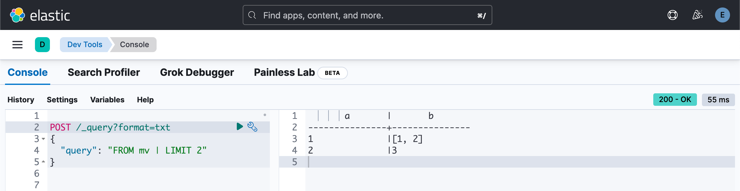
{"a":2,"b":3}

多值字段以 txt 数组的形式返回：

POST /_query?format=txt
{
  "query": "FROM mv | LIMIT 2"
}

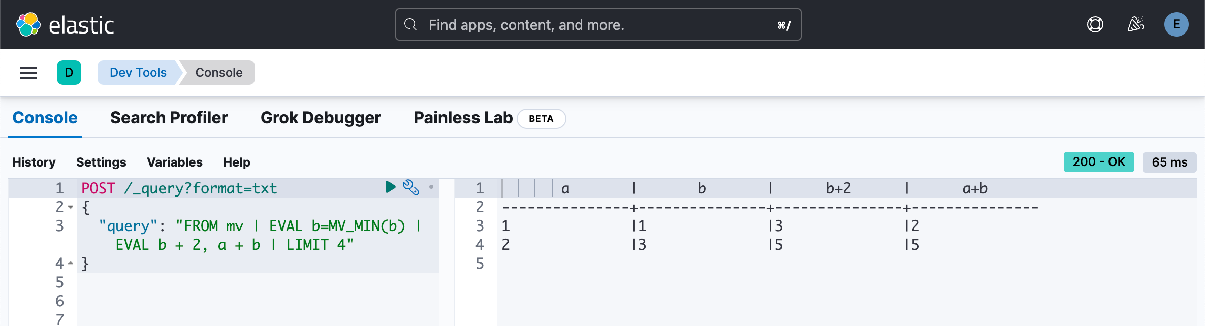
多值字段中值的相对顺序未定义。它们通常会按升序排列，但不要依赖于此。

POST /_query?format=txt
{
  "query": "FROM mv | EVAL b=MV_MIN(b) | EVAL b + 2, a + b | LIMIT 4"
}

在 Discover 中进行查询

我们可以在 Discover 中进行查询：

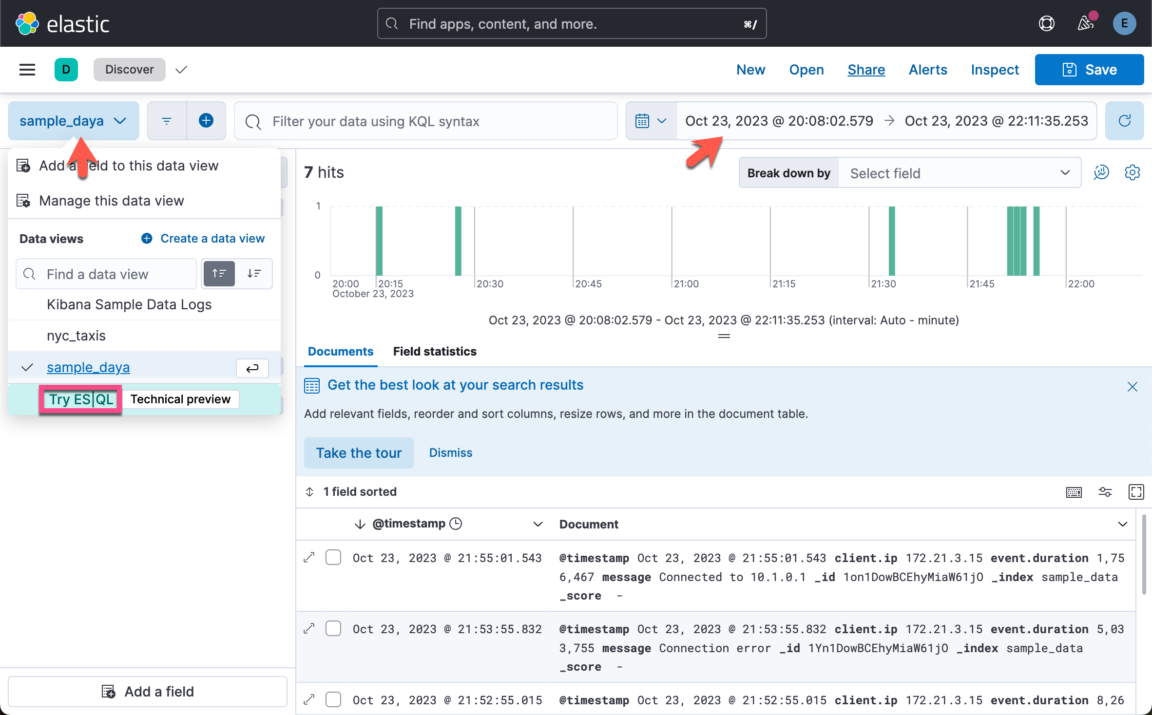
在上面，我们选择 Try ES|QL：

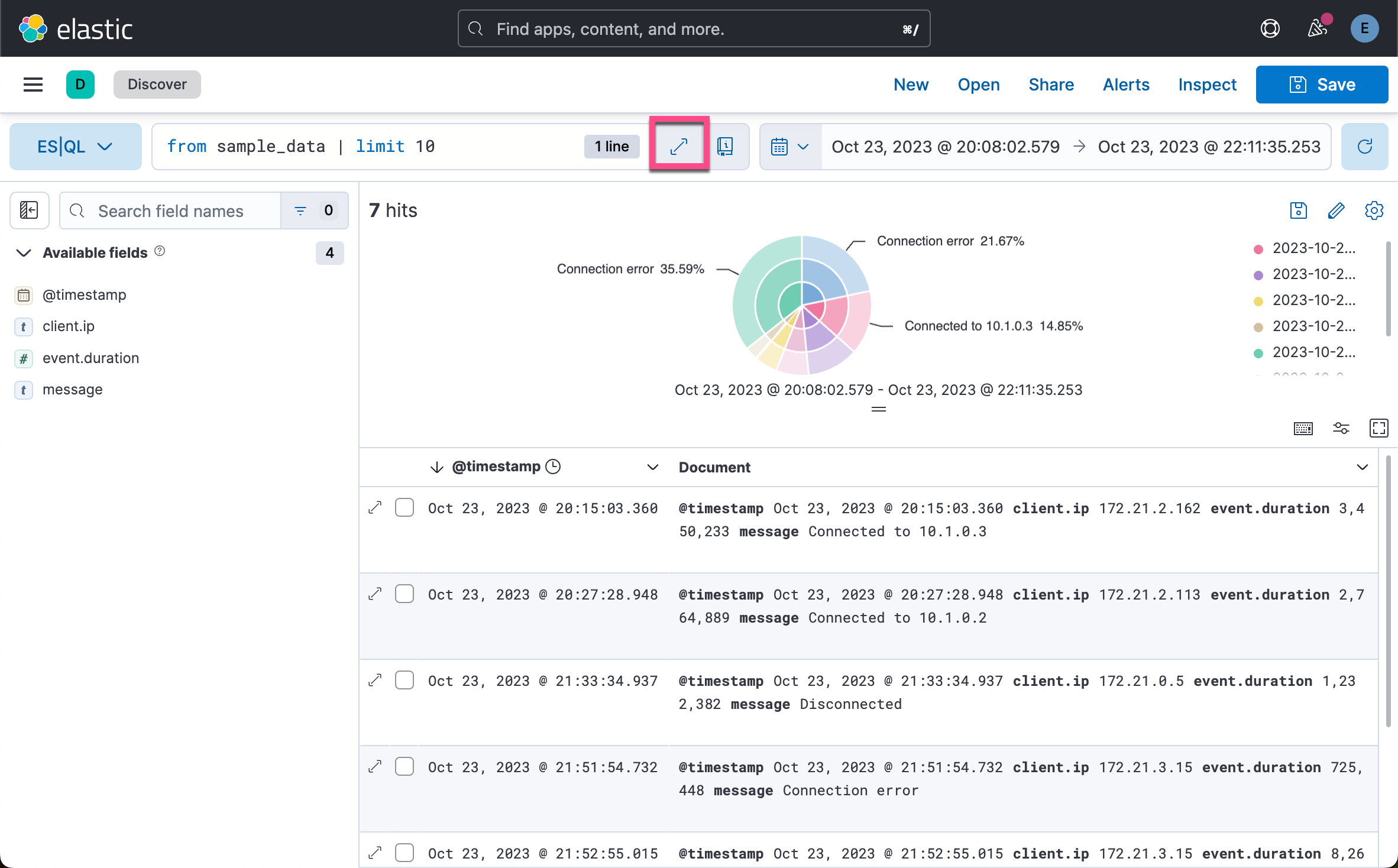
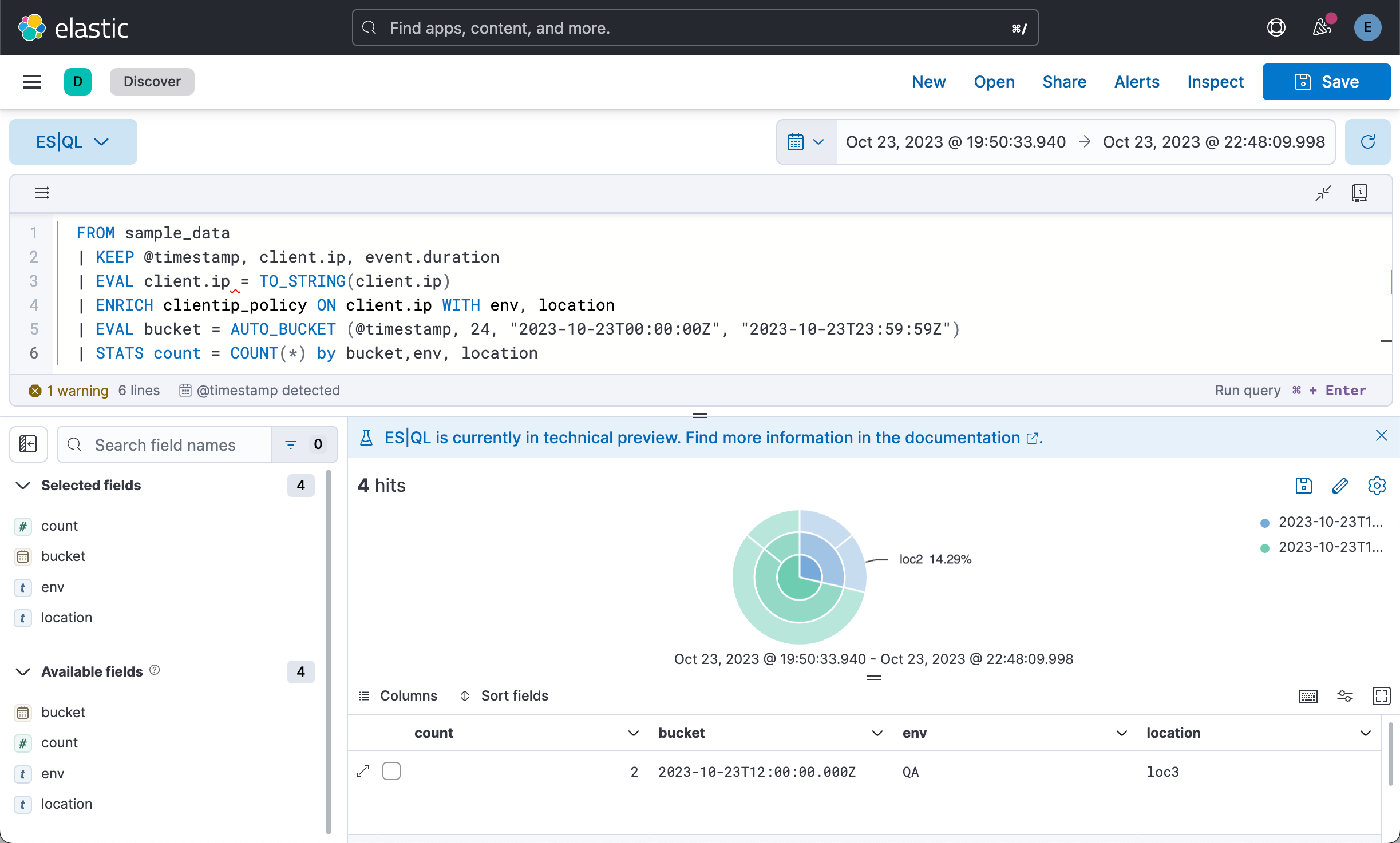
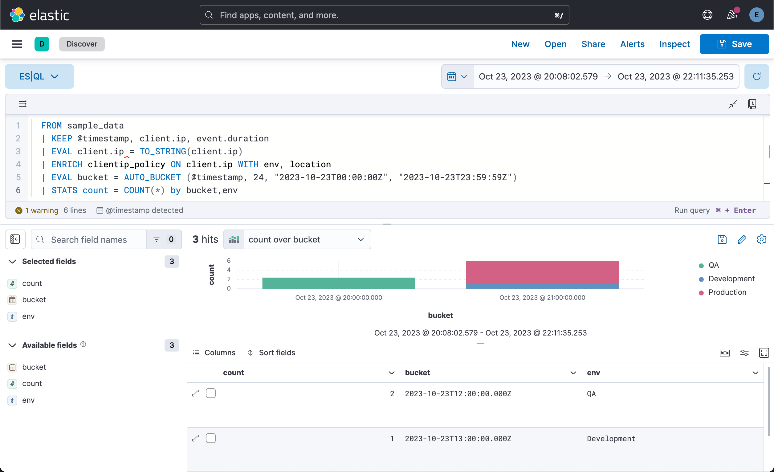
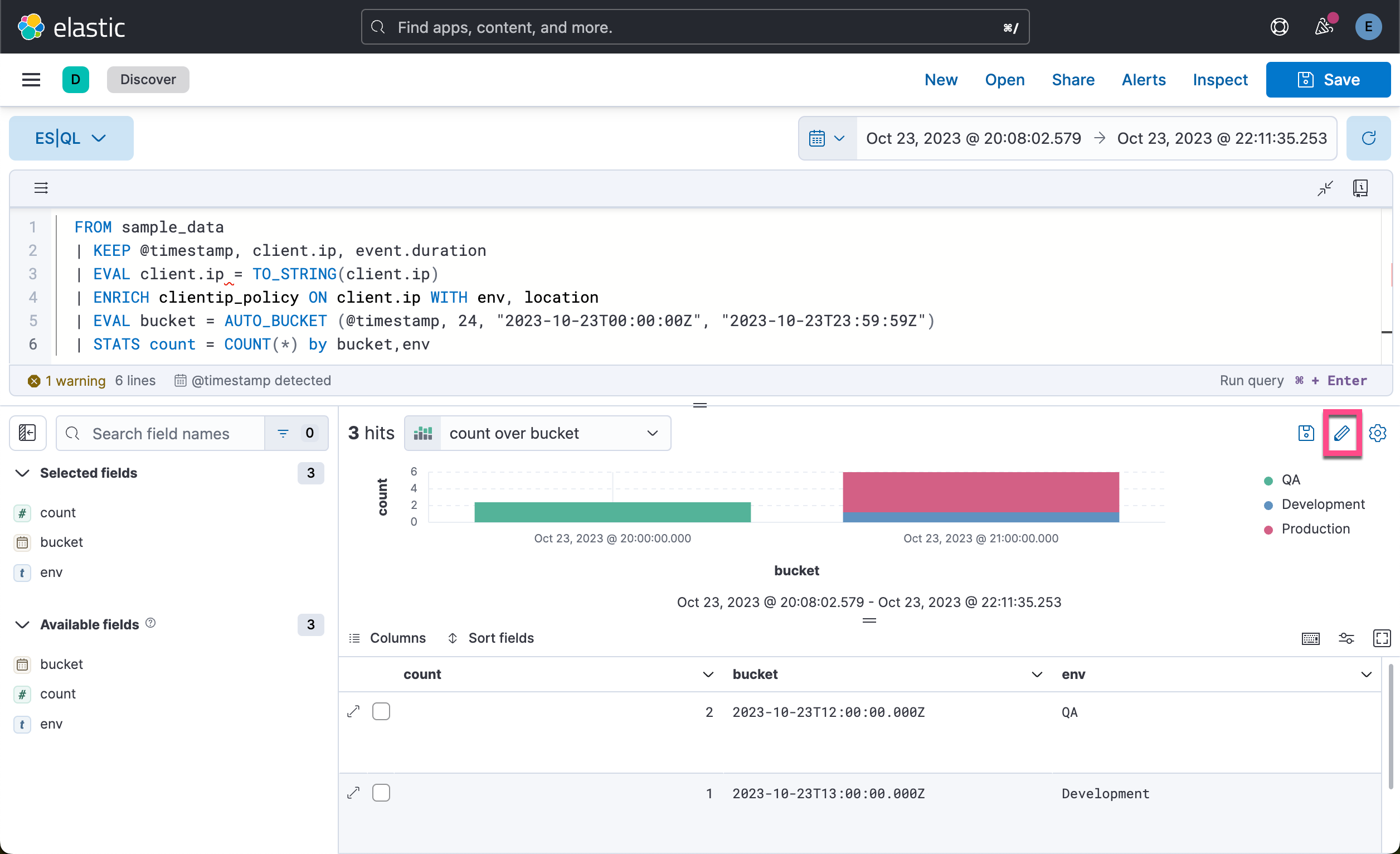
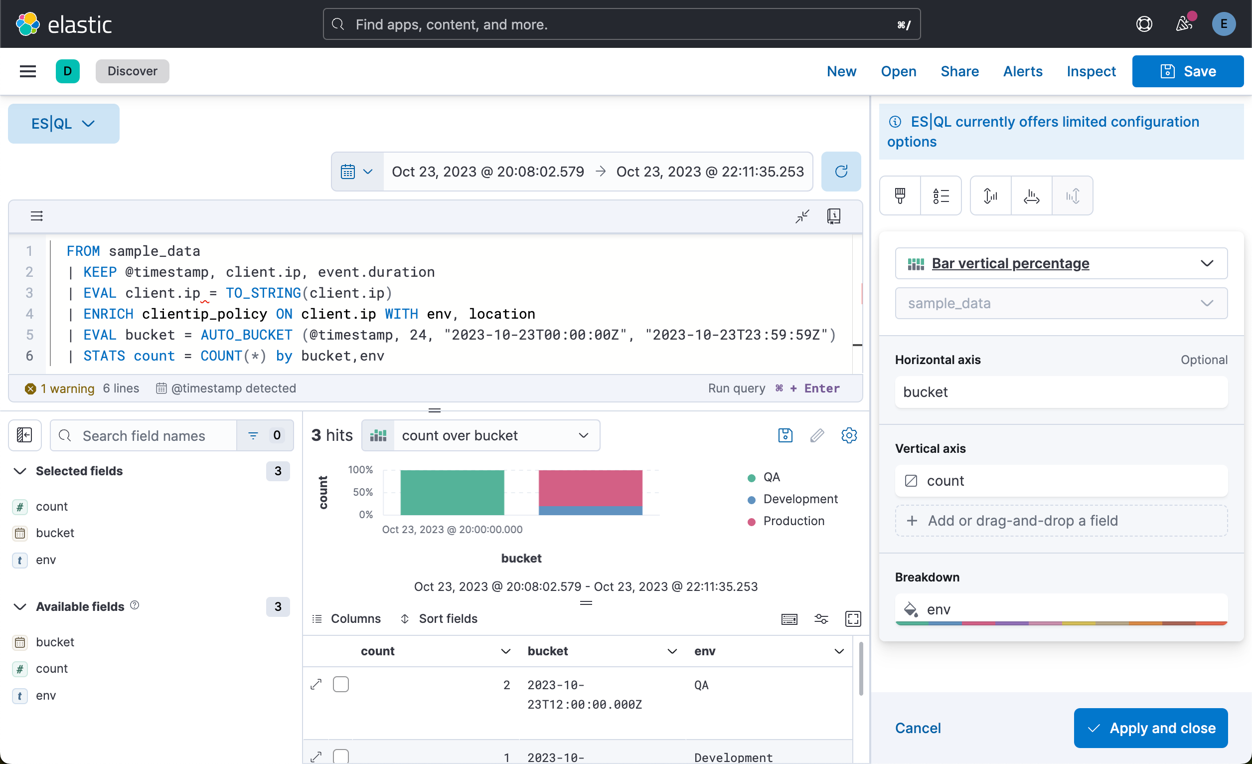
在上面，我们填入：

  FROM sample_data
  | KEEP @timestamp, client.ip, event.duration
  | EVAL client.ip = TO_STRING(client.ip)
  | ENRICH clientip_policy ON client.ip WITH env, location
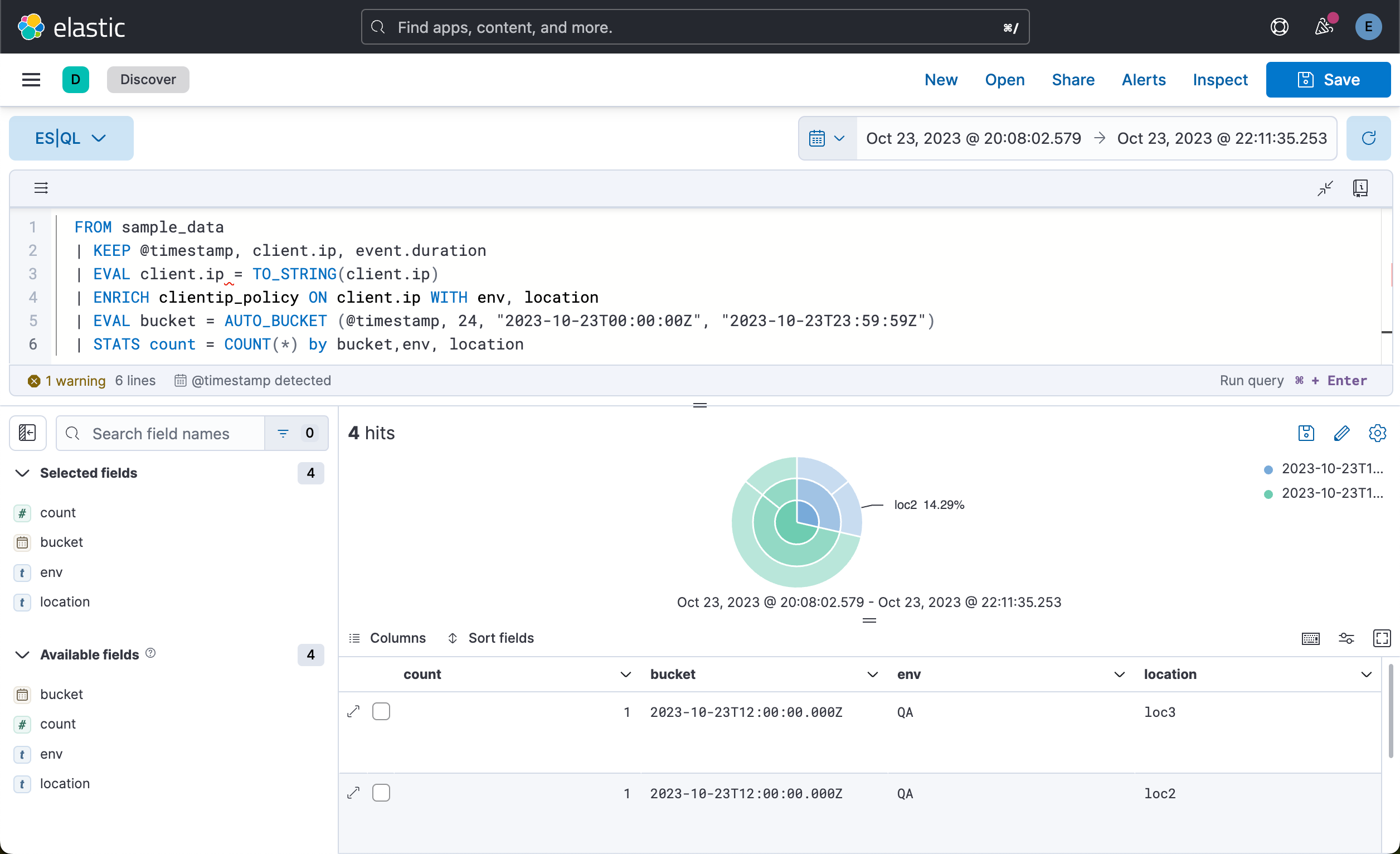
  | EVAL bucket = AUTO_BUCKET (@timestamp, 24, "2023-10-23T00:00:00Z", "2023-10-23T23:59:59Z")
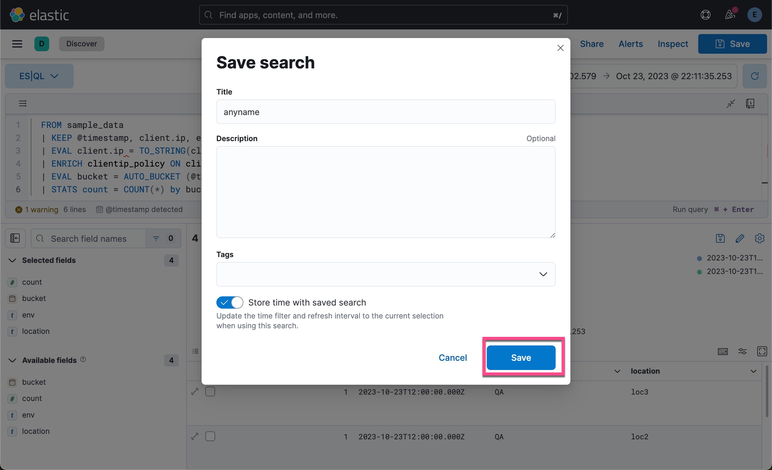
  | STATS count = COUNT(*) by bucket,env, location

我们看到的是一个可视化化图。它是一个饼图，我们可以把它保存到可视化中，并最终被 Dashboard 所示使用:

Clean up

我们可以执行如下的命令来清除之前的数据：

DELETE sample_data
DELETE clientips
DELETE /_enrich/policy/clientip_policy