一种时间序列数据的一维卷积神经网络分类方法

本文是根据阿里云天池【心跳信号分类预测】冠军攻略整理撰写，为时间序列数据的分类上提出更多解决方法。

数据集下载

登录阿里云天池，搜索心跳信号分类预测即可

赛题数据讲解

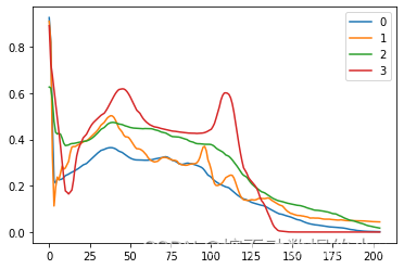
数据集均为205维的心跳时序数据，虽然是想同维度数据，很多人尝试梯度提升树，虽然说在某些方面梯度提升数类模型表现的比神经网络要好，但是这并不是绝对的，使用LGB、XGB模型需要自行构建很多特征，不能把这205维数据直接丢进去的。而神经网络则会自动寻优特征，本文就是在结构化数据分类神经网络的效果比树模型更好的一个例子。

• 主要的特征数据为 1 维信号振幅 (已被归一化至 0～1 了)，总长度均为 205 (205 个时间节点/心跳节拍)
• 除波形数据外，没有任何辅助或先验信息可以利用
• 波形数据均已被量化为 float16 类型的数值型特征，且没有类别型特征需要考虑
• 没有缺失值，无需填充，非常理想 —— 事实上，未采集到的信号默认振幅就是 0，故不存在缺失值的问题
• 这类非表格数据更适合用神经网络来处理，而非传统机器学习模型

该类别分为3类，0最多，1/2/3相对较少，可以基本判断出0为正常人心跳，1/2/3为不同心脏病病人的心跳

1.导入依赖库

import os
import math
import time
import random
import datetime
import numpy as np
import pandas as pd
import seaborn as sns
import matplotlib.pyplot as plt
import tensorflow as tf
import tensorflow.keras as K
from tensorflow.keras import Sequential, utils, regularizers, Model, Input
from tensorflow.keras.layers import Flatten, Dense, Conv1D, MaxPool1D, Dropout, AvgPool1D
from imblearn.over_sampling import SMOTE
from sklearn.model_selection import KFold
from sklearn.preprocessing import OneHotEncoder

2.数据加载

# 加载训练集和测试集(相对路径)
train = pd.read_csv('./train.csv')
test = pd.read_csv('./testA.csv')

3.数据预处理

数据精度量化压缩reduce_mem_usage(df)函数很好用，你可以在你做任何模型（图数据除外）特征工程后喂入模型前使用这个函数处理一下特征矩阵，会减少内存消耗。

# 数据精度量化压缩
def reduce_mem_usage(df):
    # 处理前 数据集总内存计算
    start_mem = df.memory_usage().sum() / 1024**2 
    print('Memory usage of dataframe is {:.2f} MB'.format(start_mem))
    
    # 遍历特征列
    for col in df.columns:
        # 当前特征类型
        col_type = df[col].dtype
        # 处理 numeric 型数据
        if col_type != object:
            c_min = df[col].min()  # 最小值
            c_max = df[col].max()  # 最大值
            # int 型数据 精度转换
            if str(col_type)[:3] == 'int':
                if c_min > np.iinfo(np.int8).min and c_max < np.iinfo(np.int8).max:
                    df[col] = df[col].astype(np.int8)
                elif c_min > np.iinfo(np.int16).min and c_max < np.iinfo(np.int16).max:
                    df[col] = df[col].astype(np.int16)
                elif c_min > np.iinfo(np.int32).min and c_max < np.iinfo(np.int32).max:
                    df[col] = df[col].astype(np.int32)
                elif c_min > np.iinfo(np.int64).min and c_max < np.iinfo(np.int64).max:
                    df[col] = df[col].astype(np.int64)  
            # float 型数据 精度转换
            else:
                if c_min > np.finfo(np.float16).min and c_max < np.finfo(np.float16).max:
                    df[col] = df[col].astype(np.float16)
                elif c_min > np.finfo(np.float32).min and c_max < np.finfo(np.float32).max:
                    df[col] = df[col].astype(np.float32)
                else:
                    df[col] = df[col].astype(np.float64)
        # 处理 object 型数据
        else:
            df[col] = df[col].astype('category')  # object 转 category
    
    # 处理后 数据集总内存计算
    end_mem = df.memory_usage().sum() / 1024**2 
    print('Memory usage after optimization is: {:.2f} MB'.format(end_mem))
    print('Decreased by {:.1f}%'.format(100 * (start_mem - end_mem) / start_mem))
    
    return df


# 训练集特征处理与精度量化
train_list = []
for items in train.values:
    train_list.append([items[0]] + [float(i) for i in items[1].split(',')] + [items[2]])
train = pd.DataFrame(np.array(train_list))
train.columns = ['id'] + ['s_' + str(i) for i in range(len(train_list[0])-2)] + ['label']  # 特征分离
train = reduce_mem_usage(train)  # 精度量化


# 测试集特征处理与精度量化
test_list=[]
for items in test.values:
    test_list.append([items[0]] + [float(i) for i in items[1].split(',')])
test = pd.DataFrame(np.array(test_list))
test.columns = ['id'] + ['s_'+str(i) for i in range(len(test_list[0])-1)]  # 特征分离
test = reduce_mem_usage(test)  # 精度量化

# 查看训练集, 分离标签与样本, 去除 id
y_train = train['label']
x_train = train.drop(['id', 'label'], axis=1)
print(x_train.shape, y_train.shape)

# 查看测试集, 去除 id
X_test = test.drop(['id'], axis=1)
print(X_test.shape)

# 将测试集转换为适应 CNN 输入的 shape
X_test = np.array(X_test).reshape(X_test.shape[0], X_test.shape[1], 1)
print(X_test.shape, X_test.dtype)

4.处理类别失衡

# 使用 SMOTE 对数据进行上采样以解决类别不平衡问题
smote = SMOTE(random_state=2021, n_jobs=-1)
k_x_train, k_y_train = smote.fit_resample(x_train, y_train)  
print(f"after smote, k_x_train.shape: {k_x_train.shape}, k_y_train.shape: {k_y_train.shape}")

# 将训练集转换为适应 CNN 输入的 shape
k_x_train = np.array(k_x_train).reshape(k_x_train.shape[0], k_x_train.shape[1], 1)

plt.hist(k_y_train, orientation = 'vertical', histtype = 'bar', color = 'blue')
plt.show() 

5.辅助函数

# 评估函数
def abs_sum(y_pred, y_true):
    y_pred = np.array(y_pred)
    y_true = np.array(y_true)
    loss = sum(sum(abs(y_pred-y_true)))
    return loss

6.模型训练与推理 (TensorFlow 2.2+)

• 由于数据特征形式较简单，仅 SMOTE 上采样处理后重复、相似性高，使用 过于复杂和深层 的神经网络将 极易过拟合，故本方案采用的模型都较为简单，且均使用了 Dropout 减轻过拟合(几乎是必须的操作)
• 模型融合并取得提升的前提是 好而不同，为此，3 个模型各自具有一定性能 (较好) 但在细节上都有一定差别 (不同)。模型的设计是本方案提升的关键，例如膨胀卷积、各种池化、分类器等，需细品
• 直接使用全数据集训练模型，训练策略均为：学习率阶梯衰减策略 LearningRateScheduler + Adam 优化器 + sparse_categorical_crossentropy 损失函数 + batch_size 64 + epoch 30

Net1

class Net1(K.Model):
    def __init__(self):
        super(Net1, self).__init__()
        # 定义4个卷积层和2个最大池化层
        self.conv1 = Conv1D(filters=16, kernel_size=3, padding='same', activation='relu', input_shape = (205, 1))
        self.conv2 = Conv1D(filters=32, kernel_size=3, dilation_rate=2, padding='same', activation='relu')
        self.conv3 = Conv1D(filters=64, kernel_size=3, dilation_rate=2, padding='same', activation='relu')
        self.conv4 = Conv1D(filters=64, kernel_size=5, dilation_rate=2, padding='same', activation='relu')
        self.max_pool1 = MaxPool1D(pool_size=3, strides=2, padding='same')
        self.conv5 = Conv1D(filters=128, kernel_size=5, dilation_rate=2, padding='same', activation='relu')
        self.conv6 = Conv1D(filters=128, kernel_size=5, dilation_rate=2, padding='same', activation='relu')
        self.max_pool2 = MaxPool1D(pool_size=3, strides=2, padding='same')
        # 定义一个dropout层和一个平铺层
        self.dropout = Dropout(0.5)
        self.flatten = Flatten()
        # 定义3个全连接层
        self.fc1 = Dense(units=256, activation='relu')
        self.fc21 = Dense(units=16, activation='relu')
        self.fc22 = Dense(units=256, activation='sigmoid')
        self.fc3 = Dense(units=4, activation='softmax')
        
    # 定义了模型的前向传播过程
    def call(self, x):
        # 连续执行4个卷积层和1个最大池化层
        x = self.conv1(x)
        x = self.conv2(x)
        x = self.conv3(x)
        x = self.conv4(x)
        x = self.max_pool1(x)
        
        # 连续执行2个卷积层和1个最大池化层
        x = self.conv5(x)
        x = self.conv6(x) 
        x = self.max_pool2(x)
        
        # 将输出进行dropout，并且平铺成一维向量
        x = self.dropout(x)
        x = self.flatten(x)
        
        # 连接两个全连接层，并将结果相加，然后再进行一次全连接操作
        x1 = self.fc1(x)
        x2 = self.fc22(self.fc21(x))
        x = self.fc3(x1+x2)
        
        return x

Net3

class GeMPooling(tf.keras.layers.Layer):
    # 定义GeM池化层类
    def __init__(self, p=1.0, train_p=False):
        super().__init__()
        self.eps = 1e-6
        # 初始化p值
        self.p = tf.Variable(p, dtype=tf.float32) if train_p else p

    def call(self, inputs: tf.Tensor, **kwargs):
        # 对输入进行裁剪，使其在[1e-6, 最大值]之间，并且求出x的p次幂
        inputs = tf.clip_by_value(inputs, clip_value_min=1e-6, clip_value_max=tf.reduce_max(inputs))
        inputs = tf.pow(inputs, self.p)
        # 对求得的值在每个通道上进行均值池化，并求出x的1/p次幂
        inputs = tf.reduce_mean(inputs, axis=[1], keepdims=False)
        inputs = tf.pow(inputs, 1./self.p)
        return inputs

# 定义了一个名为Net3的网络
class Net3(K.Model):
    def __init__(self):
        super(Net3, self).__init__()
        # 定义了多个卷积层、池化层、全连接层和dropout层
        self.conv1 = Conv1D(filters=16, kernel_size=3, padding='same', activation='relu',
                            input_shape=(205, 1))
        self.conv2 = Conv1D(filters=32, kernel_size=3, dilation_rate=2, padding='same', activation='relu')
        self.conv3 = Conv1D(filters=64, kernel_size=3, dilation_rate=2, padding='same', activation='relu')
        self.max_pool1 = MaxPool1D(pool_size=3, strides=2, padding='same')
        
        self.conv4 = Conv1D(filters=64, kernel_size=5, dilation_rate=2, padding='same', activation='relu')
        self.conv5 = Conv1D(filters=128, kernel_size=5, dilation_rate=2, padding='same', activation='relu')
        self.max_pool2 = MaxPool1D(pool_size=3, strides=2, padding='same')
        
        self.conv6 = Conv1D(filters=256, kernel_size=5, dilation_rate=2, padding='same', activation='relu')
        self.conv7 = Conv1D(filters=128, kernel_size=7, dilation_rate=2, padding='same', activation='relu')
        
        # 使用定义的GeM池化层
        self.gempool = GeMPooling()
        self.dropout1 = Dropout(0.5)
        self.flatten = Flatten()

        self.fc1 = Dense(units=256, activation='relu')
        self.fc21 = Dense(units=16, activation='relu')
        self.fc22 = Dense(units=256, activation='sigmoid')
        self.fc3 = Dense(units=4, activation='softmax')

    def call(self, x):
        # 执行多个卷积层和池化层操作，提取特征
        x = self.conv1(x)
        x = self.conv2(x)
        x = self.conv3(x)
        x = self.max_pool1(x)
        
        x = self.conv4(x)
        x = self.conv5(x)
        x = self.max_pool2(x)
        
        x = self.conv6(x)
        x = self.conv7(x)

        # 对特征进行GeM池化、dropout和平铺
        x = self.gempool(x)
        x = self.dropout1(x)
        x = self.flatten(x) 
        
        # 执行多个全连接层的操作，并且将结果相加
        x1 = self.fc1(x)
        x2 = self.fc22(self.fc21(x))
        x = self.fc3(x1 + x2)  
        
        return x

Net8

class Net8(K.Model): # 定义名为Net8的网络
    def __init__(self): # 定义构造函数
        super(Net8, self).__init__() # 调用父类的构造函数
        
        # 定义卷积层1-5，每个卷积层都有一些参数：过滤器数、核大小、填充方式、激活函数等
        # 卷积层1的输入形状为（205，1）
        self.conv1 = Conv1D(filters=16, kernel_size=3, padding='same', activation='relu',input_shape = (205, 1))
        self.conv2 = Conv1D(filters=32, kernel_size=3, padding='same', dilation_rate=2, activation='relu')
        self.conv3 = Conv1D(filters=64, kernel_size=3, padding='same', dilation_rate=2, activation='relu')
        self.conv4 = Conv1D(filters=128, kernel_size=3, padding='same', dilation_rate=2, activation='relu')
        self.conv5 = Conv1D(filters=128, kernel_size=5, padding='same', dilation_rate=2, activation='relu')
        
        # 定义最大池化层和平均池化层1
        self.max_pool1 = MaxPool1D(pool_size=3, strides=2, padding='same')
        self.avg_pool1 = AvgPool1D(pool_size=3, strides=2, padding='same')
        
        # 定义卷积层6-7
        self.conv6 = Conv1D(filters=128, kernel_size=5, padding='same', dilation_rate=2, activation='relu')
        self.conv7 = Conv1D(filters=128, kernel_size=5, padding='same', dilation_rate=2,  activation='relu')
        
        # 定义最大池化层和平均池化层2
        self.max_pool2 = MaxPool1D(pool_size=3, strides=2, padding='same')
        self.avg_pool2 = AvgPool1D(pool_size=3, strides=2, padding='same')
        
        # 定义Dropout层，率为0.5
        self.dropout = Dropout(0.5)
    
        # 定义Flatten层
        self.flatten = Flatten()
        
        # 定义全连接层1-3，每个全连接层都有一些参数：神经元数、激活函数等
        self.fc1 = Dense(units=256, activation='relu')
        self.fc21 = Dense(units=16, activation='relu')
        self.fc22 = Dense(units=256, activation='sigmoid')
        self.fc3 = Dense(units=4, activation='softmax')
            
    def call(self, x): # 定义前向传播函数
        x = self.conv1(x) 
        x = self.conv2(x)
        x = self.conv3(x)
        x = self.conv4(x)
        x = self.conv5(x)
        xm1 = self.max_pool1(x)
        xa1 = self.avg_pool1(x)
        x = tf.concat([xm1, xa1], 2) # 将xm1和xa1在第二维上进行拼接，得到输出x
        
        x = self.conv6(x) 
        x = self.conv7(x) 
        xm2 = self.max_pool2(x) 
        xa2 = self.avg_pool2(x) 

        x = tf.concat([xm2, xa2], 2) # 将xm2和xa2在第二维上进行拼接，得到输出x
        
        x = self.dropout(x) 
        x = self.flatten(x) 
        
        x1 = self.fc1(x) # 输入x经过全连接层1后得到x1
        x2 = self.fc22(self.fc21(x)) # 输入x经过全连接层2和全连接层1后得到x2
        x = self.fc3(x1+x2) # x1和x2相加后的结果进入全连接层3，得到最终的输出x
        
        return x

7.软投票融合 + 阈值法

• 由于 3 个单模均输出类别概率预测值，故使用 Soft Voting 根据 A 榜单模得分设置权重，以实现预测结果加权融合
• 由于本赛题属于分类问题，可使用阈值法将预测概率不小于 0.5 的类别置 1，其余则置 0
• 对于预测概率均小于 0.5 的难样本，使用二次处理：若最大预测值比次大预测值至少高 0.04 (这个值需要自己把握)，则认为最大预测值足够可信并置 1 其余置 0；否则认为最大预测值和次大预测值区分度不够高，难以分辨不作处理，仅令最小的另外两个预测值置 0

# 根据 A 榜得分，加权融合预测结果
predictions_weighted = 0.35 * predictions_nn1 + 0.31 * predictions_nn3 + 0.34* predictions_nn8
predictions_weighted[:5]

# 准备提交结果
submit = pd.DataFrame()
submit['id'] = range(100000, 120000)
submit['label_0'] = predictions_weighted[:, 0]
submit['label_1'] = predictions_weighted[:, 1]
submit['label_2'] = predictions_weighted[:, 2]
submit['label_3'] = predictions_weighted[:, 3]
submit.head()

# 第一次后处理未涉及的难样本 index
others = []

# 第一次后处理 - 将预测概率值大于 0.5 的样本的概率置 1，其余置 0
threshold = 0.5  
for index, row in submit.iterrows():
    row_max = max(list(row[1:]))  # 当前行中的最大类别概率预测值
    if row_max > threshold:
        for i in range(1, 5):
            if row[i] > threshold:
                submit.iloc[index, i] = 1  # 大于 0.5 的类别概率预测值置 1
            else:
                submit.iloc[index, i] = 0  # 其余类别概率预测值置 0
    else:
        others.append(index)  # 否则，没有类别概率预测值不小于 0.5，加入第一次后处理未涉及的难样本列表，等待第二次后处理
        print(index, row)

# 第二次后处理 - 在预测概率值均不大于 0.5 的样本中，若最大预测值与次大预测值相差大于 0.04，则将最大预测值置 1，其余预测值置 0；否则，对最大预测值和次大预测值不处理 (难分类)，仅对其余样本预测值置 0
for idx in others:
    value = submit.iloc[idx].values[1:]
    ordered_value = sorted([(v, j) for j, v in enumerate(value)], reverse=True)  # 根据类别概率预测值大小排序
    #print(ordered_value)
    if ordered_value[0][0] - ordered_value[1][0] >= 0.04:  # 最大与次大值相差至少 0.04
        submit.iloc[idx, ordered_value[0][1]+1] = 1  # 则足够置信最大概率预测值并置为 1
        for k in range(1, 4):
            submit.iloc[idx, ordered_value[k][1]+1] = 0  # 对非最大的其余三个类别概率预测值置 0
    else:
        for s in range(2, 4):
            submit.iloc[idx, ordered_value[s][1]+1] = 0  # 难分样本，仅对最小的两个类别概率预测值置 0        
        
    print(submit.iloc[idx])   

# 保存预测结果
submit.to_csv(("./submit_"+datetime.datetime.now().strftime('%Y%m%d_%H%M%S') + ".csv"), index=False)