左神数据结构与算法笔记-----图算法
目录
一、图的定义
定义:图是由一组顶点和一组能够将两个顶点相连的边组成的。
二、图的存储方式
假设有这样一张图
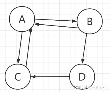
1、邻接表
表示从该点出发能到达的直接邻居列表
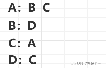
2、邻接矩阵
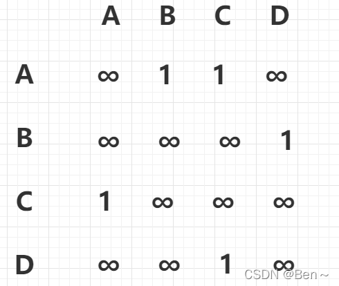
表示每个点之间的关系(∞为无法直接到达的点)
3、其他自己熟悉的方式
如通过边与点的对象存储:(出发点,终点,边的权值)
三、图的遍历
1、广度优先遍历
- 利用队列实现
- 从源节点开始依次按照宽度进队列,然后弹出
- 每弹出一个点,把该节点所有没有进过队列的邻接点放入队列
- 直到队列变空
//从Node出发,进行广度优先遍历
public class BFSTest {
	//从Node出发,进行广度优先遍历
	public static void bfs(Node node) {
		if(node==null) {
			return;
		}
		Queue<Node> queue=new LinkedList<>();
		HashSet<Node> set=new HashSet<>();	//记录已经访问过的节点,避免出现重复访问
		queue.add(node);
		set.add(node);
		while(!queue.isEmpty()) {
			Node cur=queue.poll();
			System.out.println(cur.value);
			for(Node next:cur.nexts) {	//遍历当前节点能直接到达的节点
				if(!set.contains(next)) {
					set.add(next);
					queue.add(next);
				}
			}
		}
	}
}
2、深度优先遍历
- 利用栈实现
- 从源节点开始把节点按照深度放入栈,然后弹出
- 没弹出一个点,把该节点下一个没有进过栈的邻接点发放入栈
- 直到栈变空
public class DFSTest {
	public static void dfs(Node node) {
		if(node==null) {
			return;
		}
		Stack<Node> stack=new Stack<>();
		HashSet<Node> set=new HashSet<>();
		stack.push(node);
		set.add(node);
		System.out.println(node.value);
		while(!stack.isEmpty()) {
			Node cur=stack.pop();
			for(Node next:cur.nexts) {
				if(!set.contains(next)) {
					System.out.println(next.value);
					stack.push(cur);	//先压入父节点
					stack.push(next);
					set.add(next);
					break;
				}
			}
		}
	}
}
Kruskal算法也是一种贪心算法,它是将边按权值排序,每次从剩下的边集中选择权值最小且两个端点不在同一集合的边加入生成树中,反复操作,直到加入了n-1条边。
四、图的拓扑排序
- 在图中找到所有入度为0的点输出
- 把所有入度为0的点在图中删除,继续找入度为0的点输出,周而复始
- 图的所有点删除之后,依次输出的顺序就是拓扑排序
要求:有向图且其中没有环
应用:事件安排,编译顺序
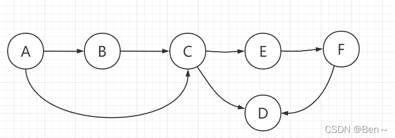
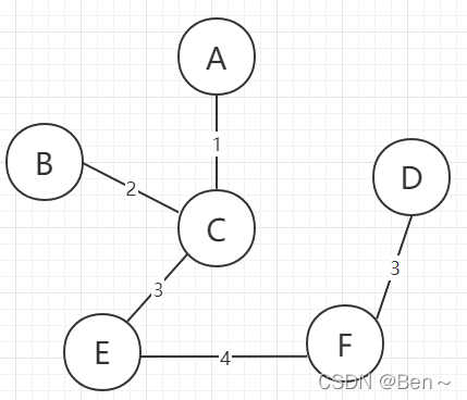
拓扑排列顺序为:A B C E F D
public class Topology {
	public static List<Node> sortedTopology(Graph graph){
		//key:某一个node
		//value:剩余的入度
		HashMap<Node, Integer> inMap=new HashMap<>();
		//入度为0的点,才能进入这个队列
		Queue<Node> zeroInQueue=new LinkedList<Node>();
		for(Node node:graph.nodes.values()) {
			inMap.put(node, node.in);
			if(node.in==0) {
				zeroInQueue.add(node);
			}
		}

		//拓扑排序的结果加入result
		List<Node> result=new ArrayList<Node>();

		while(!zeroInQueue.isEmpty()) {
			Node cur=zeroInQueue.poll();
			result.add(cur);
			for(Node next:cur.nexts) {
				inMap.put(next, inMap.get(next)-1);
				if(inMap.get(next)==0) {
					zeroInQueue.add(next);
				}
			}
		}

		return result;
	}
}
五、最小生成树
1、概念
给定一个无向图,如果他的某个子图中,任意两个顶点都能互相连通并且是一棵树,那么这棵树就叫做生成树,如果边上有权值,那么使得边权和最小的生成树叫做最小生成树。
2、kruskal算法
- 总是从权值最小的边开始考虑,依次考虑权值依次变大的边
- 当前的边要么进入最小生成树的集合,要么丢弃
- 如果当前的边进入最小生成树的集合中不会形成环,就选择当前边
- 如果当前的边进入最小生成树的集合中会形成环,就不选择当前边
- 考虑完所有的边,就得到了最小生成树
①将边以权值从小到大排序
②遍历各条边,以上述规则选择边
public class Kruskal {
	public static class EdgeComparator implements Comparator<Edge>{
		@Override
		public int compare(Edge o1, Edge o2) {
			// TODO Auto-generated method stub
			return o1.weight-o2.weight;
		}
	}

	// Union-Find Set,并查集
	public static class UnionFind {
		// key 某一个节点, value key节点往上的节点
		private HashMap<Node, Node> fatherMap;
		// key 某一个集合的代表节点, value key所在集合的节点个数
		private HashMap<Node, Integer> sizeMap;

		public UnionFind() {
			fatherMap = new HashMap<Node, Node>();
			sizeMap = new HashMap<Node, Integer>();
		}

		public void makeSets(Collection<Node> nodes) {
			fatherMap.clear();
			sizeMap.clear();
			for (Node node : nodes) {
				fatherMap.put(node, node);
				sizeMap.put(node, 1);
			}
		}
		//找到这个集合的代表
		private Node findFather(Node n) {
			Stack<Node> path = new Stack<>();
			while(n != fatherMap.get(n)) {
				path.add(n);
				n = fatherMap.get(n);
			}
			while(!path.isEmpty()) {
				fatherMap.put(path.pop(), n);
			}
			return n;
		}

		//判断两个点是否在同一个集合中
		public boolean isSameSet(Node a, Node b) {
			return findFather(a) == findFather(b);
		}

		//将两个点并入同一个集合
		public void union(Node a, Node b) {
			if (a == null || b == null) {
				return;
			}
			Node aDai = findFather(a);
			Node bDai = findFather(b);
			if (aDai != bDai) {
				int aSetSize = sizeMap.get(aDai);
				int bSetSize = sizeMap.get(bDai);
				if (aSetSize <= bSetSize) {
					fatherMap.put(aDai, bDai);
					sizeMap.put(bDai, aSetSize + bSetSize);
					sizeMap.remove(aDai);
				} else {
					fatherMap.put(bDai, aDai);
					sizeMap.put(aDai, aSetSize + bSetSize);
					sizeMap.remove(bDai);
				}
			}
		}
	}


	//用并查集实现kruskal算法
	public static Set<Edge> kruskalMST(Graph graph){
		UnionFind unionFind = new UnionFind();
		unionFind.makeSets(graph.nodes.values());
		// 从小的边到大的边,依次弹出,小根堆!
		PriorityQueue<Edge> priorityQueue = new PriorityQueue<>(new EdgeComparator());
		for (Edge edge : graph.edges) { // M 条边
			priorityQueue.add(edge);  // O(logM)
		}
		Set<Edge> result = new HashSet<>();
		while (!priorityQueue.isEmpty()) { // M 条边
			Edge edge = priorityQueue.poll(); // O(logM)
			if (!unionFind.isSameSet(edge.from, edge.to)) { // O(1)
				result.add(edge);
				unionFind.union(edge.from, edge.to);
			}
		}
		return result;
	}
}
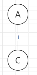
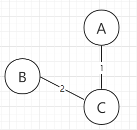
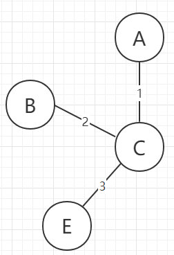
3、prim算法
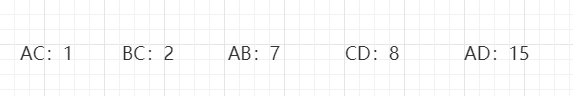
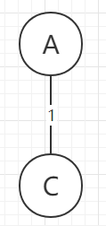
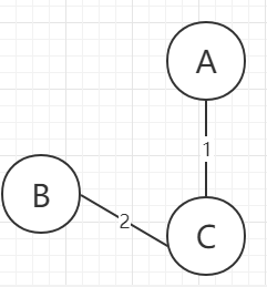
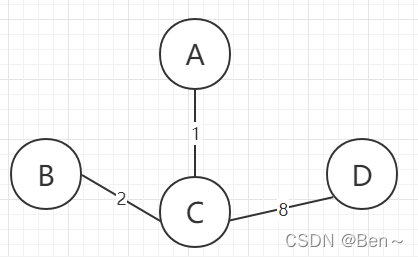
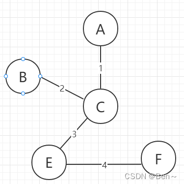
假设有这么一张图:
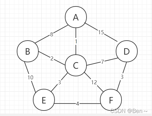
我们需要定义一个已解锁点集合nodeSet和一个已解锁边集合edgeSet
①随机选择一个点加入nodeSet中,并将与它相连的边加入edgeSet。假设我们选择了A点
②选择已解锁边集合中权值最小且边的另一个点不在已解锁点集合中,选择后将该边从已解锁边集合删除,并把另一个点加入已解锁点集合中
③重复第②步直到所有的点加入了已解锁集合
图解过程如下:
public class Prim {

	//定义一个堆比较器,将边的权值从小到大排序
	public static class EdgeComparator implements Comparator<Edge>{
		@Override
		public int compare(Edge o1, Edge o2) {
			// TODO Auto-generated method stub
			return o1.weight-o2.weight;
		}
	}

	public static Set<Edge> primSet(Graph graph){
		PriorityQueue<Edge> priorityQueue=new PriorityQueue<>(new EdgeComparator());
		//解锁出来的Node
		HashSet<Node> nodeSet=new HashSet<>();
		//解锁出来的edge
		HashSet<Edge> edgeSet =new HashSet<>();

		ArrayList<Integer> list=new ArrayList<>();
		Set<Edge> result=new HashSet<>();	//依次挑选的边放在result
		for(Node node:graph.nodes.values()) {	//随便挑了一个点,此for循环防止出现森林
			//node是开始点
			if(!nodeSet.contains(node)) {
				nodeSet.add(node);
				for(Edge edge:node.edges) {	//由该点解锁所有相关的边
					if(!edgeSet.contains(edge)) {
						priorityQueue.add(edge);
						edgeSet.add(edge);
					}
				}
				while(!priorityQueue.isEmpty()) {
					Edge edge=priorityQueue.poll();	//弹出已解锁边中的最小边
					Node toNode=edge.to;	//可能的新一个节点
					if(!nodeSet.contains(toNode)) {
						nodeSet.add(toNode);
						result.add(edge);
					}
					for(Edge nextEdge:toNode.edges) {
						priorityQueue.add(nextEdge);
					}
				}
			}
			break;
		}
		return result;
	}
}
六、最短路径
1、BFS求最短路径
bfs算法求最短路径是针对无权图而言
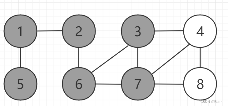
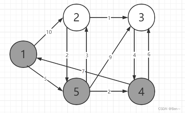
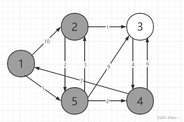
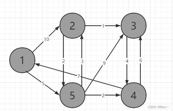
假设有这样一张图:
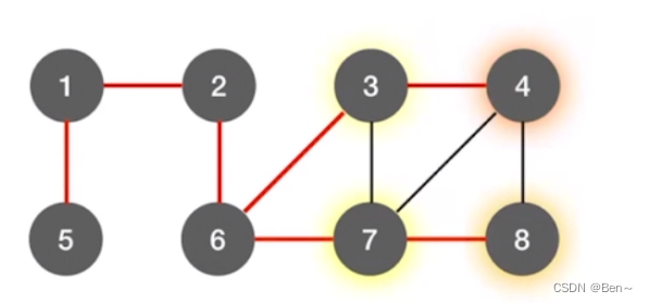
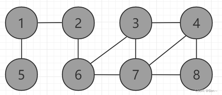
我们要求顶点2到其他各个顶点的最短路径,算法过程如下(灰色为应访问过的顶点,白色为未访问过的顶点):

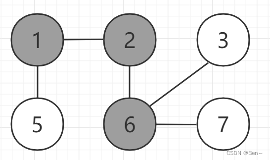
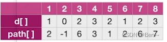
最终得出路径:
- d[]为顶点2到其他顶点的最短路径
- path[]为相应定点的前驱顶点
//求顶点u到其他顶点的最短路径
public void BFS_MIN_DISTANCE(Graph G,int u){
	int[] d=new int[Graph.vexnum];
	int[] path=new int[Graph.vexnum];
	boolean[] visited=new boolean[Graph.vexnum];
	Queue<Integer> queue=new LinkedList<>():
	for(int i=0;i<G.vexnum;i++){
		d[i]=Integer.MAX_VALUE;
		path[i]=i;
	}
	visited[u]=true;
	queue.offer(u);
	while(!queue.isEmpty()){	//bfs算法主过程
		int cur=queue.poll();
		for(int i:findNeighbor(G,cur)){
			if(!visited[i]){	//如果i没有被访问过
				d[i]=d[cur]+1;	//路径长度+1
				path[i]=cur;	//路径从cur到i
				visited[i]=true;
				queue.offer(i);
			}
		}
	}
}
2、Dijkstra算法求单源最短路径
在构造算法的过程中我们需要两个辅助数组
- dist[]:记录从源点v0到其他各顶点的最短路径长度
- path[]:path[i]表示从源点到顶点i之间的最短路径的前驱节点
算法步骤如下:
- 初始化:集合S初始为{源点},dist[]初始为dist [i]= arcs [源点] [i] (i=1,2,3,4,…)
- 从顶点集合V-S中选出vj,满足dist[j]=Min{dist[i] | vi∈V-S},此时vj就是当前求得的从v0出发的最短路径
- 修改v0到集合V-S中任意顶点vj的可达的最短路径长度,若修改后的长度小于dist[vj] 则更新为修改后的长度
- 重复2. 3.操作共n-1次,直到所有的顶点都在S中
图解:
假设有如下一张有向图,此时要求顶点1到其他定点的最短路径
S={1}
dist={0,10,∞,∞,5}

S={1,5}
dist={0,8,14,7,5}
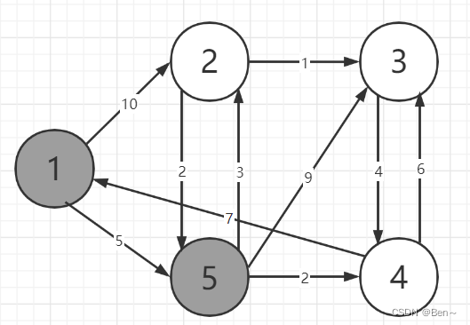
S={1,5,4}
dist={0,8,13,7,5}
S={1,5,4,2}
dist={0,8,11,7,5}
S={1,5,4,2,3}
dist={0,8,11,7,5}
代码:
public int[] getShortestPaths(int[][] adjMatrix) {
    int[] dist = new int[adjMatrix.length];   //用于存放顶点0到其它顶点的最短距离
    boolean[] visited = new boolean[adjMatrix.length];  //用于判断顶点是否被遍历
    visited[0] = true;  //假设1作为源点,表示顶点0已被遍历
    for(int i = 1;i < adjMatrix.length;i++) {	//初始化
        dist[i] = adjMatrix[0][i];
        visited[i] = false;
    }

    for(int i = 1;i < adjMatrix.length;i++) {
        int min = Integer.MAX_VALUE;    //用于暂时存放顶点0到i的最短距离,初始化为Integer型最大值
        int k = 0;
        for(int j = 1;j < adjMatrix.length;j++) {  //找到顶点0到其它顶点中距离最小的一个顶点
            if(!visited[j] && dist[j] != -1 && min > result[j]) {
                min = result[j];
                k = j;
            }
        }
        visited[k] = true;    //将距离最小的顶点,记为已遍历
        for(int j = 1;j < adjMatrix.length;j++) {  //然后,将顶点0到其它顶点的距离与加入中间顶点k之后的距离进行比较,更新最短距离
            if(!visited[j]) {  //当顶点j未被遍历时
                //首先,顶点k到顶点j要能通行;这时,当顶点0到顶点j的距离大于顶点0到k再到j的距离或者顶点0无法直接到达顶点j时,更新顶点0到顶点j的最短距离
                if(adjMatrix[k][j] != -1 && (dist[j] > min + adjMatrix[k][j] || dist[j] == -1))
                    dist[j] = min + adjMatrix[k][j];
            }
        }
    }
    return dist;
}
3、Floyd算法求各定点之间的最短路径
基本思想:
弗洛伊德算法定义了两个二维矩阵:
-
矩阵matrix记录顶点间的最小路径,例如matrix[0][3]= 10,说明顶点0 到 3 的最短路径为10;
-
矩阵pre记录顶点间最小路径中的中转点,例如pre[0][3]= 1 说明,0 到 3的最短路径轨迹为:0 -> 1 -> 3。
它通过3重循环,k为中转点,v为起点,w为终点,循环比较matrix[v][w] 和 matrix[v][k] + matrix[k][w] 最小值,如果matrix[v][k] + matrix[k][w] 为更小值,则把matrix[v][k] + matrix[k][w] 覆盖保存在matrix[v][w]中。注意:k≠v,v≠w。
public class Graph {
	private char[] vertex;
	private int[][] matrix;
	private int[][] pre;

	public Graph(char[] vertex,int[][] matrix) {
		this.vertex=vertex;
		this.matrix=matrix;
		pre=new int[matrix.length][matrix.length];
	}

	//初始化图
	public void init() {
		for(int i=0;i<vertex.length;i++) {
			Arrays.fill(pre[i], i);
		}
	}

	//弗洛伊德算法
	public void flyd() {
		int m=0;
		for(int k=0;k<vertex.length;k++) {	//k为中间节点
			for(int i=0;i<vertex.length;i++) {
				for(int j=0;j<vertex.length;j++) {
					if(i==j) {
						continue;
					}
					m=matrix[i][k]+matrix[k][j];
					if(m<matrix[i][j]) {
						matrix[i][j]=m;	//更新最短路径
						pre[i][j]=pre[k][j];	//更新中间节点
					}
				}
			}
		}
	}
}
4、三种最短路径算法比较
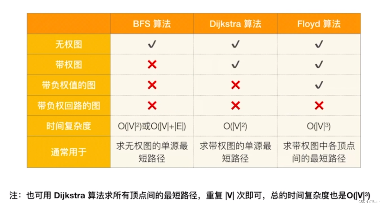
参考博文:
最小生成树
弗洛伊德(Floyd)算法求图的最短路径