[2201] VRT: A Video Restoration Transformer

paper
supp
code

Abstract

video restoration methods

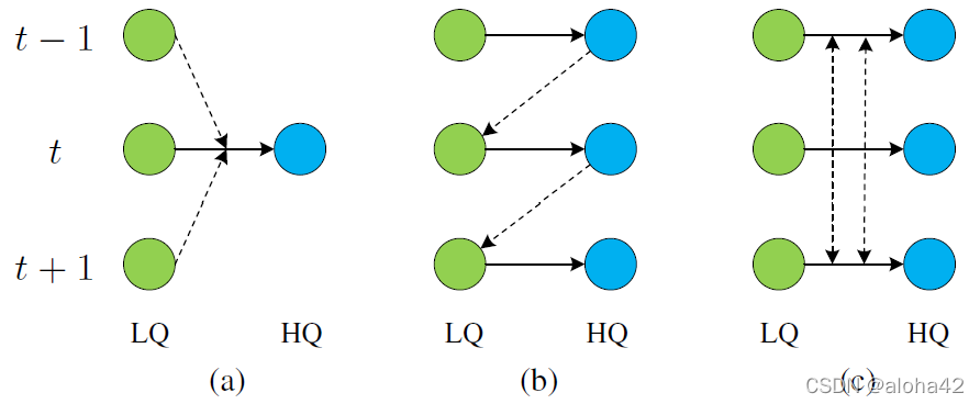
• sliding window-based method
  input multiple LQ frames to generate a single HQ frame
  each input frame processed for multiple times in inference
  $⟹$ inefficient feature utilization and increased computation cost
• recurrent method
  use previously reconstructed HQ frames for subsequent frame reconstruction
  3 drawbacks due to recurrent nature
  • limited in parallelization
  • poor at long-range temporal dependency modelling
    $⟸$ one frame strongly affect the next frame, but its influence quickly lost after few time steps
  • significant performance drop on few-frame videos
• parallel method
  divide video sequence into non-overlapping clips and shift it alternately to enable inter-clip interactions

Illustrative comparison of sliding window-based models, recurrent models and the proposed parallel VRT model. Green and blue circles denote low-quality (LQ) input frames and high-quality (HQ) output frames, respectively. $t-1$, $t$ and $t+1$ are frame serial numbers. Dashed lines represent information fusion among different frames.

contributions

• propose Video Restoration Transformer (VRT)
  • parallel computation, long-range dependency modelling
  • jointly extract, align, fuse frame features at multiple scales
• propose multi-head mutual attention (MMA)
  • mutual alignment between frames
• SOTA on video restoration
  • video SR, video deblurring, video denoising

Method

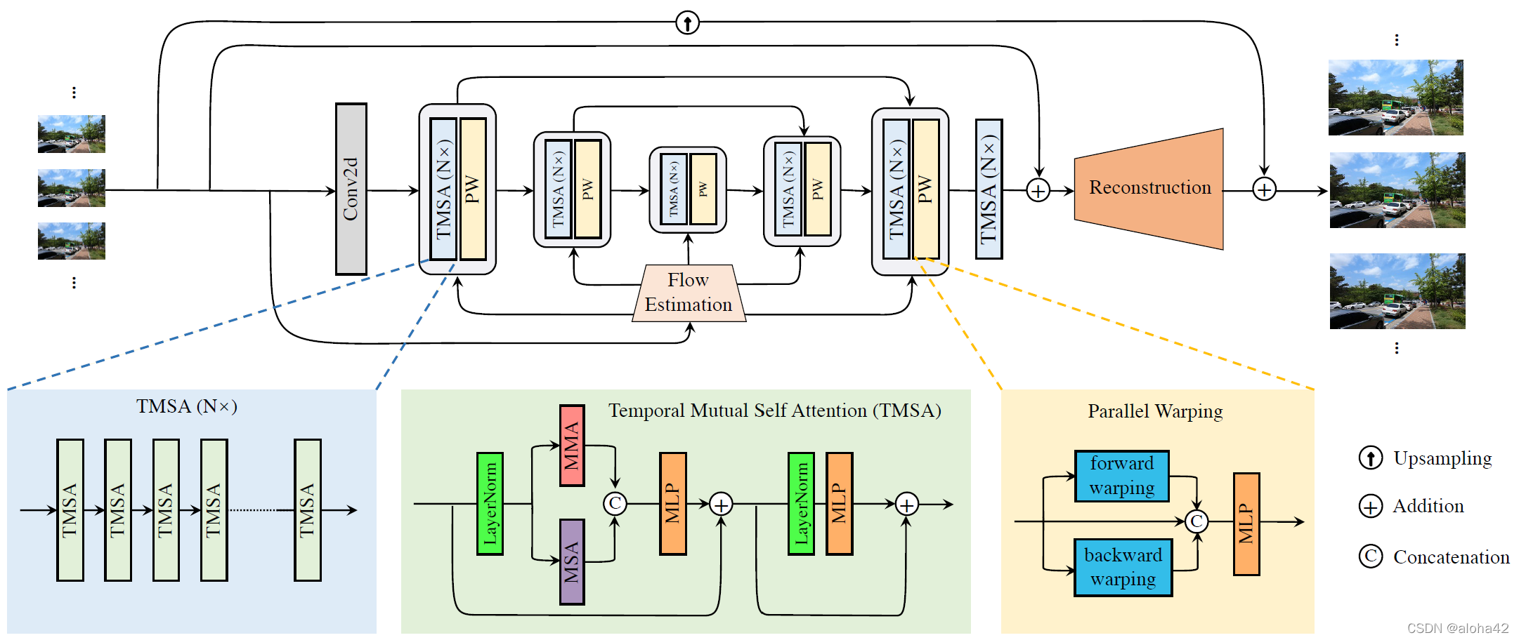
model architecture

The framework of the proposed Video Restoration Transformer (VRT). Given T low-quality input frames, VRT reconstructs T high-quality frames in parallel. It jointly extracts features, deals with misalignment, and fuses temporal information at multiple scales. On each scale, it has two kinds of modules: temporal mutual self attention (TMSA) and parallel warping. The down-sampling and up-sampling operations between different scales are omitted for clarity.

given a sequence of low-quality input frames $I^{LQ}\in {\mathbb{R}}^{T\times H\times W\times C_{in}}$, a sequence of high-quality target frames $I^{HQ}\in {\mathbb{R}}^{T\times sH\times sW\times C_{out}}$
where, $s$ is upscaling factor: $s>1$ for sr, $s=1$ for db and dn
aim to restore $T$ HQ frames from $T$ LQ frames in parallel for various video restoration tasks

feature extraction
extract shallow features $I^{SF}\in {\mathbb{R}}^{T\times H\times W\times C}$ from $I^{LQ}$ by a conv
propose a multi-scale network that aligns frames at different resolutions based on U-Net
capture features and motions at different scales by TMSA and PW, where skip connections added for features of same scales
add TMSA for further feature refinement to obtain deep features $I^{DF}\in {\mathbb{R}}^{T\times H\times W\times C}$

reconstruction
restore HQ frames $I^{RHQ}\in {\mathbb{R}}^{T\times sH\times sW\times C}$ from addition of shallow feature $I^{SF}$ and deep feature $I^{DF}$

• sr: sub-pixel conv with upscale factor $s$
• db, dn: single conv

loss function Charbonnier loss
between reconstructed HQ sequence $I^{RHQ}$ and ground-truth HQ sequence $I^{HQ}$
$$\mathcal{L}=\sqrt{\Vert I^{RHQ}-I^{HQ}{\Vert }^2+{ϵ}^2}$$

where, $ϵ$ is a constant, empirically set as 1e-3

temporal mutual self attention (TMSA)

Illustrations for mutual attention and temporal mutual self attention (TMSA). In (a), we let the orange square (the $i$-th element of the reference frame) query elements in the supporting frame and use their weighted features as a new representation for the orange square. The weights are shown around solid arrows (we only show three examples for clarity). When $A_{i,k}\to 1$ and the rest $A_{i,j}\to 0(j\ne k)$, the mutual attention equals to warping the yellow square to the position of the orange square (illustrated as a dashed arrow). (b) shows a stack of temporal mutual self attention (TMSA) layers. The sequence is partitioned into 2-frame clips at each layer and shifted for every other layer to enable cross-clip interactions. Dashed lines represent information fusion among different frames.

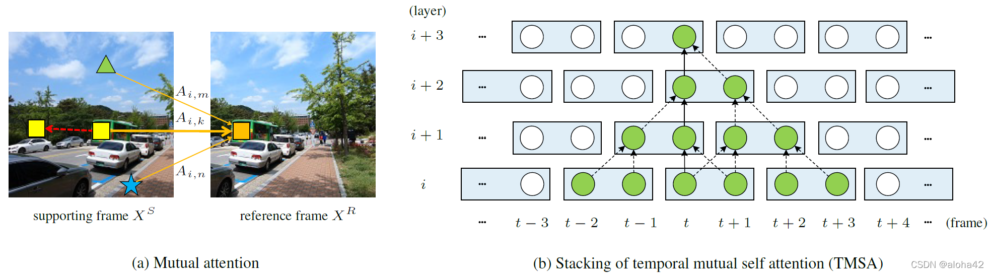
mutual attention

given reference frame features $X^R\in {\mathbb{R}}^{N\times C}$, neighboring frame features $X^S\in {\mathbb{R}}^{N\times C}$
compute query, key, value by linear projection
$$\begin{array}{rl}{Q}^R& =X^R{P}^Q\\ K^S& =X^S{P}^K\\ V^S& =X^S{P}^V\end{array}$$

where, $P^Q,P^K,P^V\in {\mathbb{R}}^{C\times D}$ are projection matrices, $N$ is feature elements number, $D$ is channels number of projected features
use $Q^R$ to query $K^S$ to generate attention features for weighed sum of $V^S$
$$MA(Q^R,K^S,V^S)=softmax(\frac{Q^R(K^S{)}^T}{\sqrt{D}})V^S$$

rewrite equation for $i$-th element in reference frame
$$Y_{i,:}^R=\sum _{j=1}^{N}Ai,j{V}_{j,:}^S$$

where, $Y_{i,:}^R$ is the new features of $i$-th element in reference frame, $A\in {\mathbb{R}}^{N\times N}$ is attention features reflecting correlations between reference and neighboring frame

$K_{k,:}^S$ (yellow box in fig.a) is the most similar element to $Q_{i,:}^R$ (orange box in fig.a), and $K_{j,:}^S(j\ne k)$ are dissimilar to $Q_i^R$
$$A_{i,k}>A_{i,j},\forall j\ne k,j\le N$$

$$\{\begin{array}{ll}{A}_{i,k}\to 1& \text{, }\\ A_{i,j}\to 0& \text{, }\forall j\ne k,j\le N\end{array}$$

combining above equations, have
$$Y_{i,:}^R=V_{k,:}^S$$

$⟹$ move $k$-th element in neighboring frame to the position of $i$-th element in reference frame (red arrow in fig.a)
$⟹$ image warping given an optical flow vector

in practice, reference frame and neighboring frame can be exchanged, allowing mutual alignment between those 2 frames
similar to MSA, perform attention for $h$ times and concatenate results as multi-head mutual attention (MMA)

benefits of mutual attention

• preserve information from neighboring frames adaptively
  avoid “black hole” artifacts
• no inductive biases of locality
  inherent to most CNN-based motion estimation
  performance drop when 2 neighboring objects move towards different directions
• conduct motion estimation and warp on features in a joint way
  optical flows only estimated on RGB image and not robust

temporal mutual self attention

combine mutual attention with self-attention
given $X\in {\mathbb{R}}^{2\times N\times C}$represent 2 frames
split $X$ into 2 part of features
$$X_1,X_2=spli{t}_0(LN(X))\in {\mathbb{R}}^{1\times N\times C}$$

where, $split(\cdot )$ is an operator on 0-dimension
apply MMA on $X_1,X_2$ for 2 times: warp $X_1$ towards $X_2$, warp $X_2$ towards $X_1$
$$\begin{array}{rl}{Y}_1& =MMA(X_1,X_2)\\ Y_2& =MMA(X_2,X_1)\end{array}$$

combine warped features and concatenate with MSA result
$$Y=conca{t}_0(conca{t}_2(Y_1,Y_2),MSA(X))$$

where, $conca{t}_0(\cdot ),conca{t}_2(\cdot )$ are operators on 0- and 2-dimension
feed $Y$ into 2 consecutive MLP with skip connection
$$\begin{array}{rl}X& =MLP(Y)+X\\ X& =MLP(LN(X))+X\end{array}$$

only 2 frames dealt at a time $⟸$ design of mutual attention
extend for $T$ frames: deal with frame-to-frame pairs exhaustively
$⟹$ complexity $\mathcal{O}(T^2)$

solution inspired by shifted-window mechanism in Swin
step 1 partitions video sequence into non-overlapping 2-frame clips, and apply MMA-MSA to each clip in parallel
step 2 shift sequence temporally by 1 frame for every other layer (in fig.b) to enable cross-clip connections
$⟹$ complexity $\mathcal{O}(T)$

temporal receptive field size increase when multiple TMSA modules stacked together
at layer $\ell (\ell \ge 2)$, one frame utilize information from up to $2(\ell -1)$ frames

parallel warping (PW)

spatial window partition $⟹$ mutual attention unable to deal with large motions well
solution use feature warping at the end of each stage

Illustration of parallel warping. For every frame feature $X_t(t\le T)$, frame $X_{t-1}$ and $X_{t+1}$ are warped towards $X_t$ as ${\hat{X}}_{t-1}$ and ${\hat{X}}_{t+1}$, respectively. Then, $X_t$, ${\hat{X}}_{t-1}$ and ${\hat{X}}_{t+1}$ are concatenated together (denoted by blue boxes) for feature fusion and dimension reduction with a multi-layer perception (MLP). The final output is ${\bar{X}}_t$. The dashed arrows and circles denote warping operations and warped features, respectively.

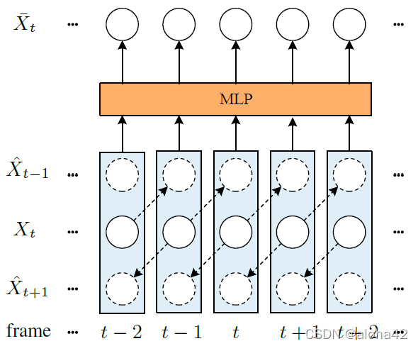
given frame $X_t$ and neighboring frames $X_{t-1},X_{t+1}$
step 1 calculate optical flows $O_{t-1,t},O_{t+1,t}$ from $X_t$ and $X_{t-1},X_{t+1}$
step 2 use $O_{t-1,t},O_{t+1,t}$ to warp $X_t$ to obtain initial warped features $X_{t-1}^{\prime },X_{t+1}^{\prime }$
$$\begin{array}{rl}{X}_{t-1}^{\prime }& =warp(X_{t-1},O_{t-1,t})\\ X_{t+1}^{\prime }& =warp(X_{t+1},O_{t+1,t})\end{array}$$

step 3 predict offset residuals $o_{t-1,t},o_{t+1,t}$ and modulation masks $m_{t-1,t},m_{t+1,t}$
$$o_{t-1,t},o_{t+1,t},m_{t-1,t},m_{t+1,t}=\mathcal{C}([O_{t-1,t},O_{t+1,t},X_{t-1}^{\prime },X_{t+1}^{\prime }])$$

where, $\mathcal{C}(\cdot )$ is a convolution layer, $[\cdot ]$ is a concatenation operator
step 4 warp $X_{t-1},X_{t+1}$ with results above
$$\begin{array}{rl}{\hat{X}}_{t-1}& =\mathcal{D}(X_{t-1},O_{t-1,t}+o_{t-1,t},m_{t-1,t})\\ {\hat{X}}_{t+1}& =\mathcal{D}(X_{t+1},O_{t+1,t}+o_{t+1,t},m_{t+1,t})\end{array}$$

where, $\mathcal{D}(\cdot )$ is a deformable convolution layer
step 5 concatenate $X_t,{\hat{X}}_{t-1},{\hat{X}}_{t+1}$ and feed into an MLP layer for ${\bar{X}}_t$ with reduced dimension

Experiment

dataset

	resolution	training set	testing set	usage
REDS	$1280\times 720$	266 clips	REDS4 4 clips	video super resolution (BI) video deblurring
Vimeo-90K	$448\times 256$	64,612 clips	Vimeo-90K-T 7,824 clips	video super resolution (BI, BD)
Vid4	$720\times 480$		4 clips each 34 frames	video super resolution
UDM10	$1272\times 720$		4 clips each 32 frames	video super resolution
DVD	$1280\times 720$	61 clips 5,708 frames totally	10 clips 1,000 frames totally	video deblurring
GoPro	$1280\times 720$	22 clips 2,103 frames totally	11 clips 1,111 frames totally	video deblurring
DAVIS	$854\times 480$	90 clips	30 clips	video denoising
Set8	$960\times 540$		8 clips each 85 frames	video denoising
experiment detail

• data augmentation random flipping, random rotation, random cropping
• input
  • sr on REDS: $64\times 64$-size, 6 or 16 frames
  • sr on Vimeo-90K: $64\times 64$-size, 7 frames
  • db, dn: $192\times 192$-size, 6 frames
• degradation
  • sr: bicubic down-sampling (BI), blur down-sampling (BD)
  • db: motion blur
  • dn: Gaussian noise $\sigma \in [0,50]$
• optimizer Adam: ${\beta }_1=0.9,{\beta }_2=0.99$, batch size=8, 300K iterations
• learning rate initial 4e-4, cosine decay

video super resolution

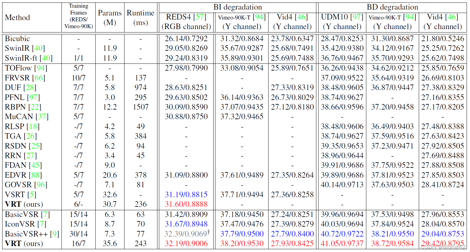
Quantitative comparison (average PSNR/SSIM) with state-of-the-art methods for video super-resolution ($\times 4$) on REDS4, Vimeo-90K-T, Vid4 and UDM10. Best and second best results are in red and blue colors, respectively. “$†$” We currently do not have enough GPU memory to train the fully parallel model VRT on 30 frames.

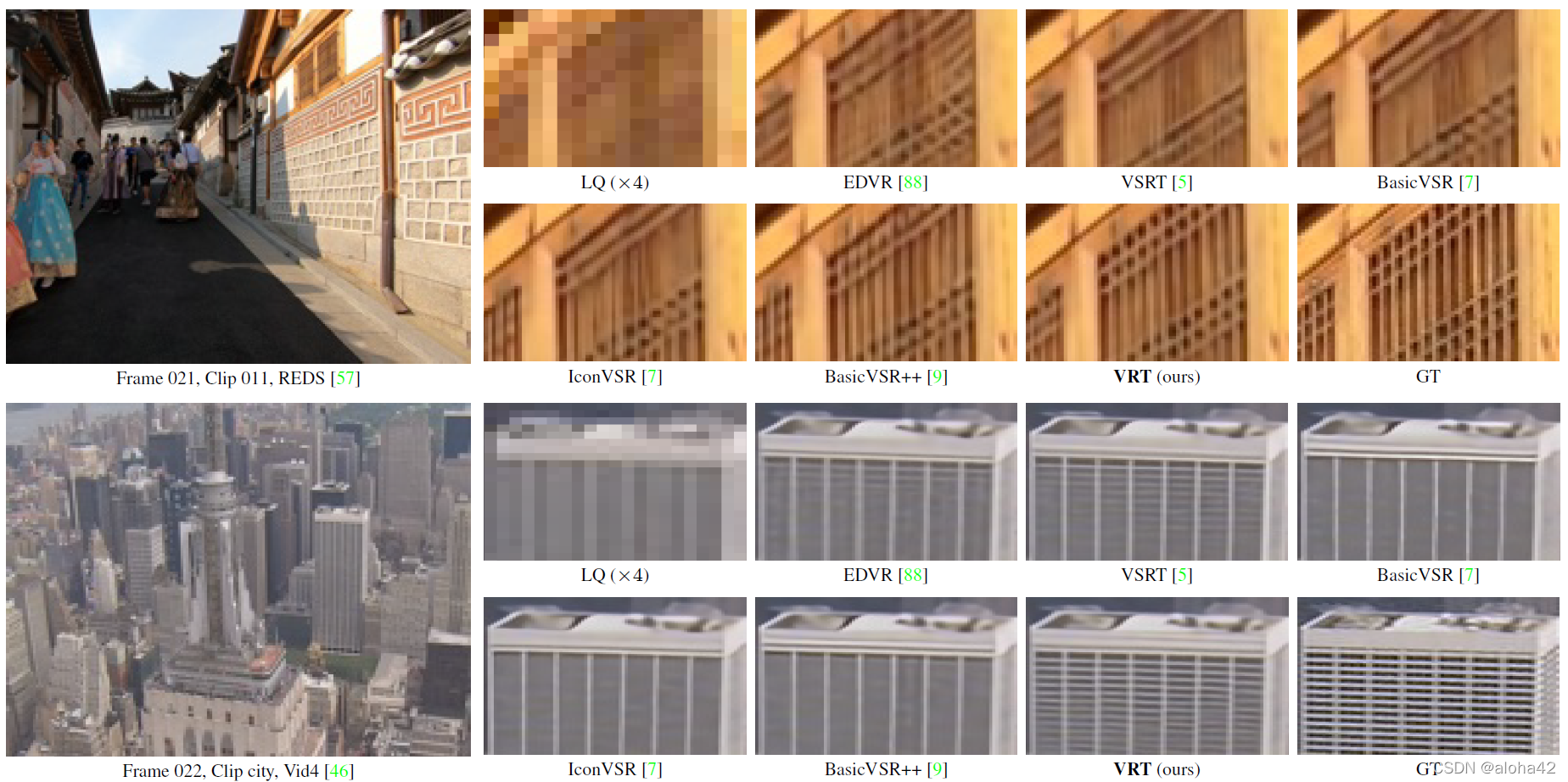
Visual comparison of video super-resolution ($\times 4$) methods.

video deblurring

Quantitative comparison (average RGB channel PSNR/SSIM) with state-of-the-art methods for video deblurring on DVD. Best and second best results are in red and blue colors, respectively.

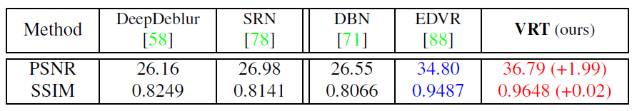
Quantitative comparison (average RGB channel PSNR/SSIM) with state-of-the-art methods for video deblurring on GoPro. Best and second best results are in red and blue colors, respectively.

Quantitative comparison (average RGB channel PSNR/SSIM) with state-of-the-art methods for video deblurring on REDS. Best and second best results are in red and blue colors, respectively.

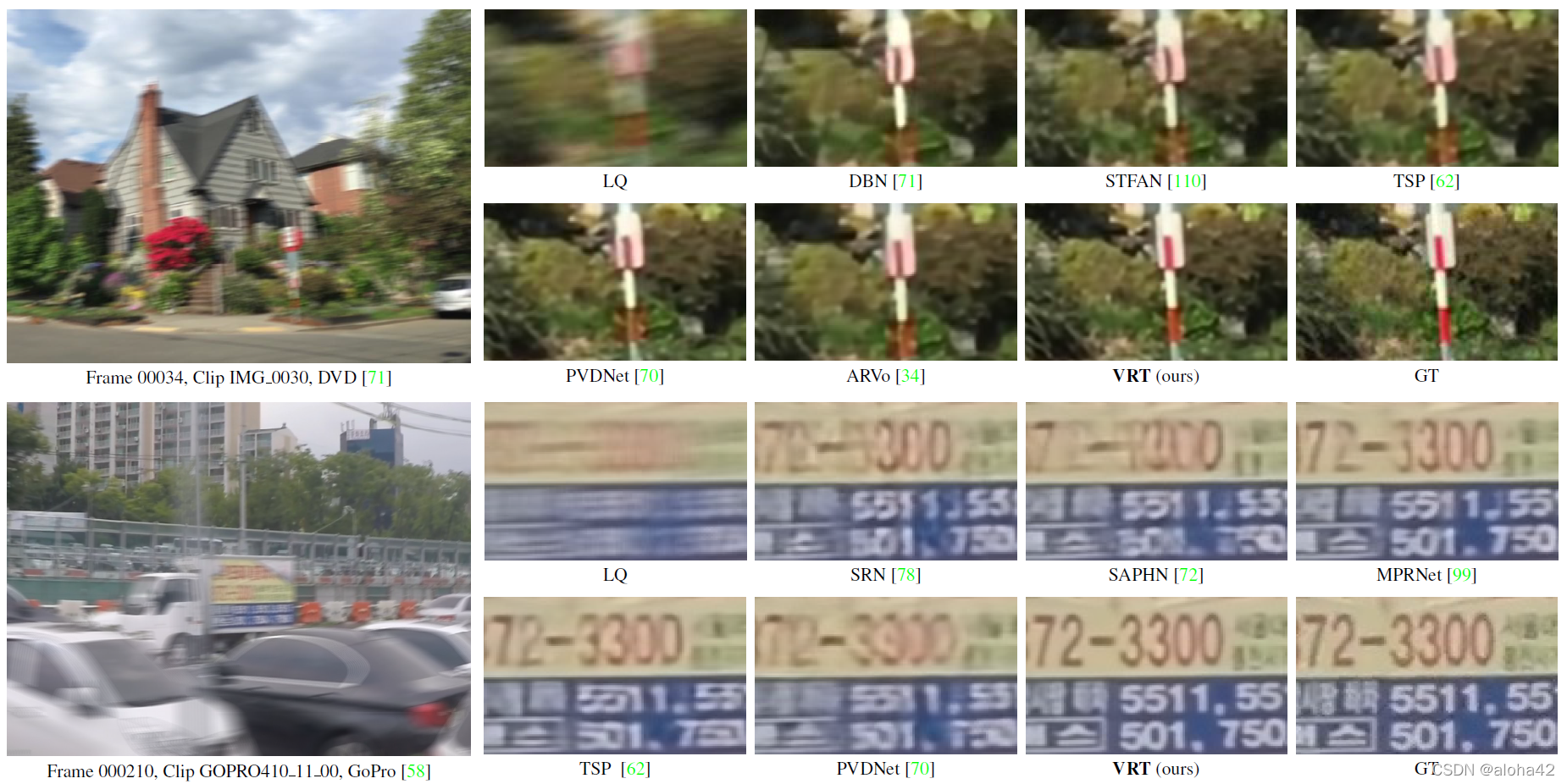
Visual comparison of video deblurring methods.

video denoising

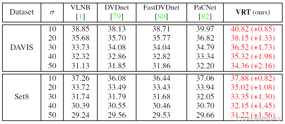
Quantitative comparison (average RGB channel PSNR) with state-of-the-art methods for video denoising on DAVIS and Set8. $\sigma$ is the additive white Gaussian noise level. Best and second best results are in red and blue colors, respectively.

ablation study

baseline a small version of VRT: layers and channels number halved

multi-scale architecture & parallel warping

Ablation study on multi-scale architecture and parallel warping. Given an input of spatial size $64\times 64$, the corresponding feature sizes of each scale are shown in brackets. When some scales are removed, we add more layers to the rest scales to keep similar model size.

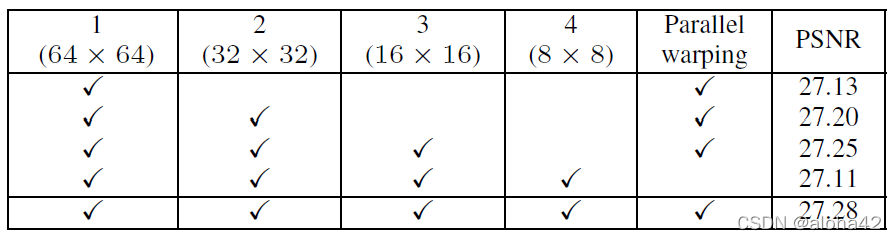
key findings

• when number of model scales reduced, performance drop gradually
  $⟸$ multi-scale processing help to utilize information from a larger area and deal with large motions between frames
• parallel warping bring an improvement of 0.17dB

temporal mutual self attention

Ablation study on temporal mutual self attention.

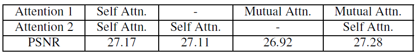
key findings

• when replace MA with SA or only use SA, performance drop by 0.11 to 0.17dB, for
  • SA focus more on reference frame rather than on neighboring frame during computation of attention
  • MA attend to neighboring frame and benefit from feature fusion
• only using MA is not enough
  $⟸$ MA cannot preserve information of reference frames

attention window size

Ablation study on attention window size (frame$\times$height$\times$width).

study window size on temporal dimension in the last several TMSA layers of each scale

• when window size increase from 1 to 2, performance improve slightly
  $⟸$ previous TMSA layers already utilize neighboring 2-frame information well
• when window size increase to 8, see an obvious improvement of 0.18dB
  $⟹$ use window size of $8\times 8\times 8$ for those layers