python数学建模导论1.3非线性规划及其python实现

python数学建模导论1.3非线性规划及其python实现

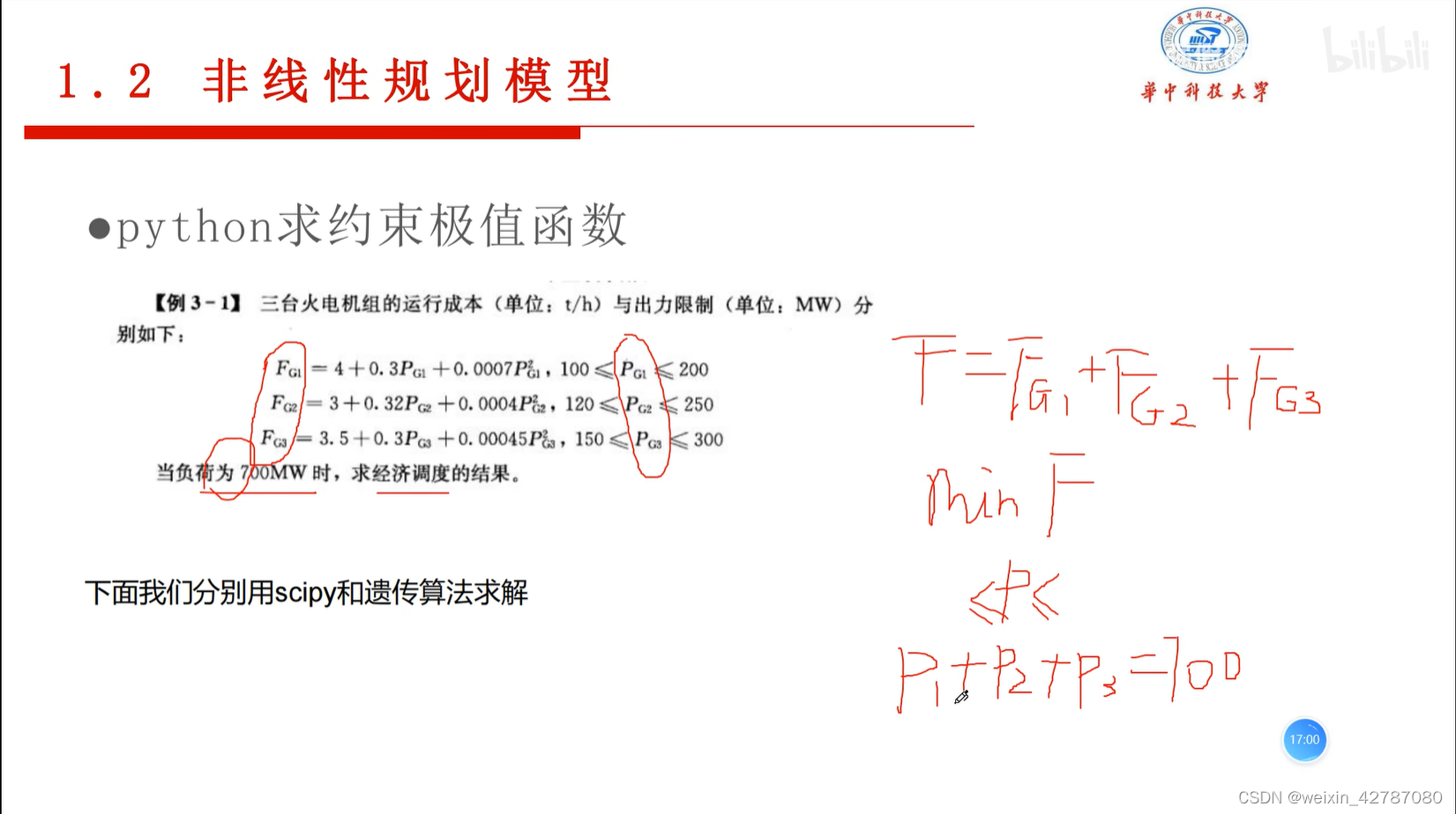
使用scipy求解

from scipy.optimize import minimize
import numpy as np

# 目标函数即min(FG1+FG2+FG3)
def fun(x):
    return (4 + 0.3 * x[0] + 0.0007 * x[0] ** 2 + 3 + 0.32 * x[1] + 0.0004 * x[1] ** 2 + 3.5 + 0.3 * x[
        2] + 0.00045 * x[2] **2)

def con():
    # 约束条件 分为eq 和ineq
    # eq表示 函数结果等于e; ineg 表示 表达式大于等于0
    cons = ({'type':'eq', 'fun':lambda x:x[0]+x[1]+x[2]-700})
    # ['type':ineq'，'fun': lambda x: -x[2] + x2max]#如果有不等式约束
    #cons=([con1，con2，con3，con4， con5，con6，con7，con8])
    #如果有多个约束，则最后返回结果是这个#x[0] 其中的e 必须是具体数字，不能是t 等参数

#上下限约束
b1=(100,200)
b2=(120,250)
b3=(150,300)
bnds = (b1,b2,b3)   #边界约束

if __name__ == '__main__':
    cons = con()  # 约束
    # 设置x初始猜测值
    x0 = np.array((150, 250, 20))
    res = minimize(fun, x0, method='l-bfgs-b', constraints=cons, bounds=bnds)
    print("代价",res.fun)
    print(res.success)
    print("解",res.x)

遗传函数方法：

from sko.GA import GA
def fun(x):
    return (4 + 0.3 * x[0] + 0.0007 * x[0] ** 2 + 3 + 0.32 * x[1] + 0.0004 * x[1] ** 2 + 3.5 + 0.3 * x[
        2] + 0.00045 * x[2] **2)
cons = lambda x:x[0]+x[1]+x[2]-700
b1=(100,200)
b2=(120,250)
b3=(150,300)
ga = GA(func=fun,n_dim=3,size_pop=500,max_iter=500,constraint_eq=[cons],lb=[100,120,150],ub=[200,250,300])
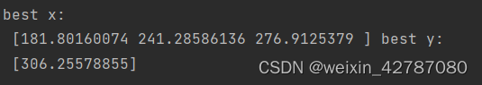
best_x,best_y = ga.run()
print("best x:\n", best_x, "best y: \n", best_y)
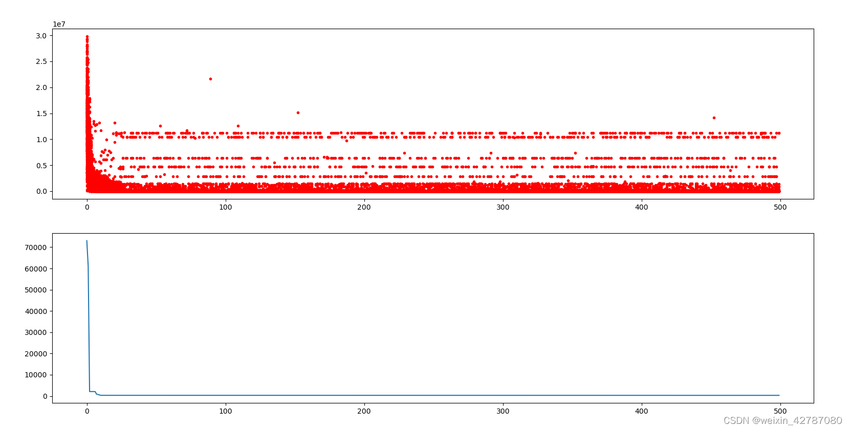
# %% Plot the result
import pandas as pd
import matplotlib.pyplot as plt
Y_history = pd.DataFrame(ga.all_history_Y)
fig, ax = plt.subplots(2,1)
ax[0].plot(Y_history.index, Y_history.values, ".", color="red")
Y_history.min(axis=1).cummin().plot(kind='line')
plt.show()